Multi-Tenant Smart Locker Capacity Management with Deep Reinforcement Learning
A deeper look into multi-tenant smart locker capacity management proposing a Deep Reinforcement learning approach to overbooking, in order to maximize throughput while keeping failure rates low.
Smart parcel locker networks are becoming increasingly essential components of logistics infrastructure. Parcel carriers rely more and more on the upkeep, reliability, and efficiency of smart locker networks as a core part of their delivery logistics.
With this growing importance of smart lockers, it's essential to provide service of highest quality, optimizing the utilization of the limited compartment space a locker can provide.
However, a parcel locker only has so many compartments available, and extensions are often costly or impossible.
If capacity is already at its limit, this defines a capacity management problem.
Smart Locker Capacity Management
Smart locker capacity management can be defined as a sequential decision-making problem. Each acceptance or rejection of an announcement impacts future states of the locker, with two main uncertainties:
- Parcel Lag: The unknown time between announcement and delivery.
- Parcel Dwell: The unknown time between delivery and collection.
A poorly managed locker may:
- Over-accept, leading to failed deliveries when compartments are full later on
- Over-reject, underutilizing available space and therefore reducing throughput
The goal is to maximize successful deliveries while minimizing failures as to efficiently utilize the limited capacity.
Challenges in Decision-Making
Due to the sequential nature of the problem, it is difficult to assess whether a decision is correct or incorrect at the time of announcement. An acceptance can lead to several outcomes:
- The parcel arrives (after others have been collected) and is delivered successfully.
- The parcel is accepted but remains pending for a long time, affecting past and future decisions.
- The parcel is delivered, but remains in the locker unusually long, affecting past and future decisions.
- The parcel arrives while the locker is full, and the delivery fails. Expected demand and estimated capacity needs change, affecting past and future decisions.
Consequently, the value of an acceptance or rejection decision cannot be determined at the time of the announcement, but must be inferred from later operational outcomes.
A successful delivery does not necessarily indicate that the historical acceptance decision was optimal. It reflects the overall strategy's success, but the reward cannot be attributed to a single decision.
Similarly, a failed delivery does not imply the acceptance was bad. Prior or subsequent decisions may have created a state in which the acceptance could not be fulfilled, even if the decision was well-justified at the time it was made.
Different Perspectives
To dive deeper into this problem, we should distinguish between two different types of locker network operators
- A multi-tenant locker network operator
- A single-tenant locker network operator
A single-tenant smart locker network operator benefits from vertical integration, enabling deeper integration with its sole tenant. This setup allows for the use of richer parcel information and tighter process integration. By serving its own network, the operator can leverage details such as a parcel's operational state, expected route, delivery attempts, and driver schedules to make more precise predictions.
A multi-tenant smart locker provider has to integrate multiple tenants into a single coherent system. To achieve this, generalization must occur at the information exchange boundary, at which data may be lost, omitted, sparse, inconsistent, or erroneous. It has little to no visibility into the couriers internal parcel state, the route that is being taken or the delivery schedules of delivery drivers.
What remains consistent, however, is the ability to receive a delivery announcement at one time, observe a drop-off at another, and later record a collection. Additional details may be available for some tenants but not others, and the quality of such information is likely to vary.
These contrasting positions create interesting profiles
- A vertically integrated network may have richer information but relatively consistent parcel flows since it serves a single underlying process.
- A multi-tenant network may have less information, but can observe different tenant behaviour and try to exploit their differences as it serves multiple different but unknown underlying processes.
Multi-Tenant: An Illustrative Example
Let's briefly define 2 types of exemplary tenants.
- General Purpose Carrier announces parcels Monday to Friday, rarely but still some on Saturday and some on Sunday. Deliveries occur 1 to 3 days after announcement, exclusively Monday through Friday, between 7 and 15 o'clock. Collections happen somewhere between 1 and 2 days after delivery (e.g., online shopping)
- Overnight Shipping Carrier announces parcels Monday through Sunday, deliveries happen mostly in the night after announcement, or early in the morning up until 9 o'clock. Collections likely happen at the day of delivery. (e.g. ordering critical medicine)
It's Friday 20:00, the locker is physically at maximum capacity, with all compartments containing a delivered parcel waiting for collection.
Scenario 1: The overnight shipment carrier requests a compartment.
Should this request be accepted? Likely not, we know from prior encounters with the overnight shipping carrier it delivers likely in the night after the announcement or latest in the morning. Chances that no-one has yet picked up a parcel of the delivered ones are high, as it's already late evening.
One might opt to reject this request.
Scenario 2: The general purpose carrier requests a compartment.
Should this request be accepted? Based on prior encounters with this tenant, the delivery is not going to happen before Monday, and the collection profile of the parcels which are currently delivered suggest collections over the weekend to be very likely. Those collections free up compartments, which would make it feasible to accept this parcel as, once it arrives, compartment space should likely be available again.
One might opt to accept this request.
The two announcement scenarios have the same current physical state but different future risk profiles.
They should not necessarily receive the same decision.
Related Work
Sequential accept/reject decision-making for parcel lockers under uncertain pickup timing is an active research area.
 Samyukta Sethuraman
Amazon Locker Capacity Management by Sethuraman et al. address a closely related problem within Amazon's own locker network: package dwell time is predicted from historical data, and the resulting forecasts feed a linear program that reserves capacity per shipping class. Their setting benefits from vertical integration, dwell-time behaviour is tied to a small, fixed set of known shipping options. The paper explicitly names strategic overbooking, similar in spirit to airline or hotel yield management, as an interesting direction it does not pursue.
 Daniela Sailer
In Dynamic Demand Management for Parcel Lockers, Sailer, Klein & Steinhardt study a single-locker acceptance problem with heterogeneous customer types and unknown pickup times, solved via a cost/value function approximation. Customer types and their governing probability distributions are given as known model inputs. Like Sethuraman et al., they name overbooking as a compelling but unaddressed extension of their feasibility-based acceptance rule.
In Dynamic stochastic parcel locker assignment with uncertain pick-up times by Mancini & Gansterer, they address a related but distinct multi-locker assignment problem, training a MIP-based linear classifier to imitate decisions of a full-information oracle. Their setting is built around a fixed, known typology (premium vs. standard customers).
Reinforcement Learning
The sequential nature of the multi-tenant smart locker capacity management problem gives rise to defining it using a reinforcement learning formulation
- State: The current locker state and the historical information available about tenant delivery and collection behaviour
- Action: Accepting or rejecting a parcel currently requesting a compartment for future delivery
- Transition: Incoming deliveries of accepted parcels, as well as collections of delivered parcels change the locker state inbetween decisions
- Reward: Accepting / Rejecting a parcel might not be easily quantifyable, but delayed reward signals allow to inferr the trajectory of the overall strategy
The objective is therefore not to perfectly predict every delivery, but to improve upon acceptance and rejection decisions under uncertainty.
Scoping the Experiment
Real world locker networks contain many optimization problems, and capacity management under high demand is just one of them.
Real systems need to account for various compartment sizes, hardware defects of the locker as a whole or just at a compartment level. They need to deal with challenging first-mile dynamics of customers showing up unannounced, compartment-to-parcel fit decisions, software ergonomics for couriers as well as customers, failing processes at the tenants end, malfunctioning component firmware, etc.
This experiment shall be deliberately limited in scope to focus on the core challenge at hand, therefore it models
- A single locker
- Equally sized compartments throughout the locker layout
- Announcement based dynamics only (last-mile + customer dispatch with announcement)
- No abandoned or uncollected parcels
- No retry of failed deliveries
The goal is to retain the difficult part of the problem while avoiding a system so broad that it becomes impossible to identify which component is responsible for a result.
Synthetic Environment
As mentioned before, there is no dataset available that labels the optimal accept/reject decision for every possible locker situation.
Even with a real dataset, the optimal counterfactual decision would not necessarily be labelled, which is however the important one:
What would have happened if the system had accepted a parcel it historically rejected? Or conversely, if it rejected a parcel it historically accepted?
The first step is therefore to create a controllable simulated environment.
In this environment, every parcel follows a causal life cycle
$$\text{Announcement} \rightarrow \text{Accept / Reject} \rightarrow \text{Delivery} \rightarrow \text{Collection}$$
An announcement creates a decision point. If the policy accepts it, the parcel becomes an accepted pending commitment. It does not occupy a physical compartment yet, but it should still influence future decisions because it will occupy one later.
When the delivery event occurs, one of two things happens:
- If a compartment is available, the parcel becomes physically delivered and occupies the locker.
- If the locker is full, the delivery fails and the parcel never creates physical occupancy.
After a successful delivery, the parcel remains in the locker until its collection event. Collection releases the compartment.
The environment and its decision points are event-driven, meaning the policy is only able to act at announcement events. An accepted parcel stays accepted, there is no possibility to retroactively reject it, it's a standing commitment.
Between the current and upcoming announcement, the environment advances through all scheduled deliveries and collections. The reward returned by one step can therefore include rewards from several automatic operational events that happened after the action and before the next decision point.
Parcel Generators
Each parcel generator represents a type of logistics tenant. Its job is to produce a causally valid parcel life cycle with an announcement timestamp, a delivery timestamp, and a collection timestamp.
The environment mixes parcels from the configured generators according to configurable probabilities.
General Purpose Parcel Generator
Simulates a typical e-commerce parcel workflow of customers ordering goods and getting them delivered after some time later.
Announcement hours are weighted toward business hours from 8 to 21 o'clock, peaking before lunch and in the afternoon. Weekday announcements follow a weighted distribution where Tuesday accounts for 25%, Wednesday and Thursday 20% each, Monday and Friday 15% each, and weekends 5% combined.
Deliveries generally occur between 8 and 17 o'clock with a morning bias, weekend deliveries are deferred to Monday. However, they are again split into 4 subtypes of General Purpose Parcel Generators, sharing same announcement and collection behaviour, but different delivery lag profiles.
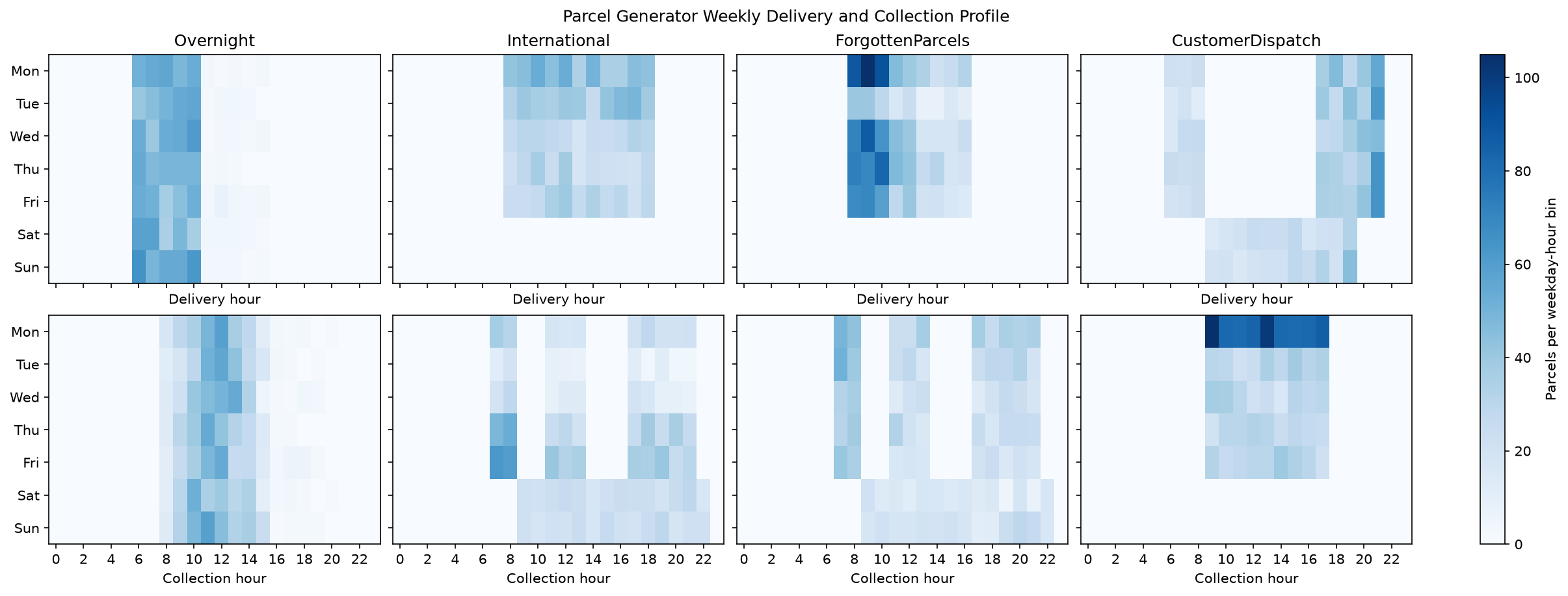
Collections for deliveries before 9 o'clock happen on the same day, either between 13 to 15 or 16 to 21, uniformly on weekdays. Deliveries after 9 o'clock are collected next day, which happens uniformly either between 6 to 10, 11 to 15 or 16 to 21 o'clock on weekdays. Next day collections for weekend collections happen uniformly between 10 to 19 o'clock.
Yearly seasonality yields a shift upwards in December, starting in November and ending in January with slight variations throughout the year.
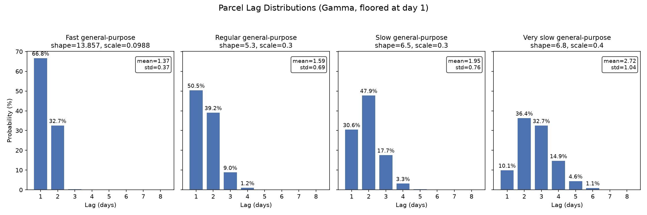
Fast General Purpose Parcel Generator
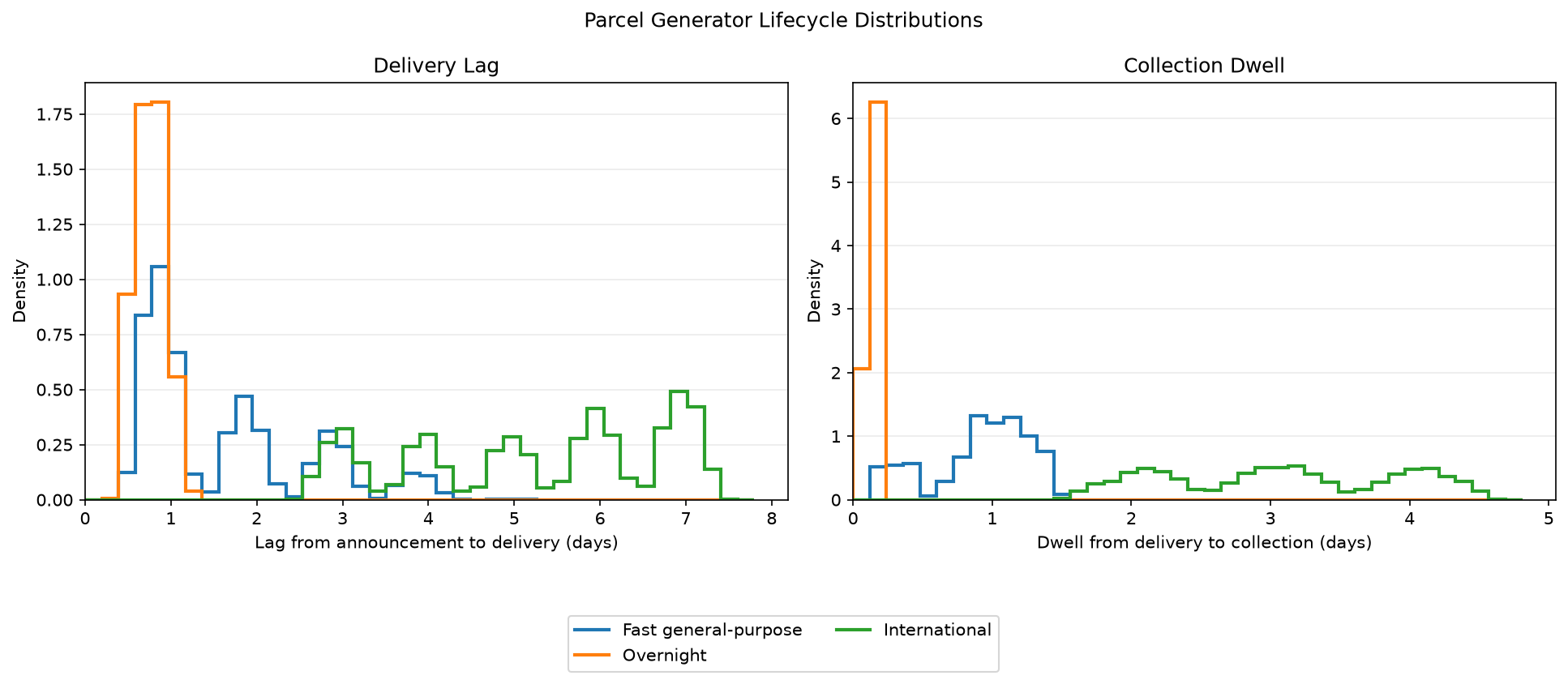
Deliveries are distributed as such that 66% of parcels are delivered after 1 day, 33% after 2 days and 1% after 3 days of announcement. Weekend delivery delays however shift them farther into the future.
Regular General Purpose Parcel Generator
Represents a dependable and consistent parcel courier, just a little less than the fast one. 50% of the parcels are delivered after 1 day, 40% after 2 days, and 10 percent after 3 days.
Weekend delays also shift deliveries farther into the future.
Slow General Purpose Parcel Generator
This type simulates a tenant which does some additional logistics in between announcement and delivery, hence parcels arrive rarer on day 1 and more often on day 2.
With a distribution of 31% arriving 1 day after announcement, 48% arriving after 2 days of announcement, 18% arriving after 3 days of announcement, 3% after 4 days. (Weekend delays also shift deliveries farther into the future)
Very Slow General Purpose Parcel Generator
Represents a challenging delivery courier in terms of predictability, with deliveries spread out over 5 days after announcement.
With 10% likelihood of a parcel arriving after 1 day, 36% after 2 days, 33% after 3 days, 15% after 4 days, 5% after 5 days and 1% after 6 days.
Similarly, deliveries scheduled for the weekend are delayed to the next weekday, moving them even farther into the future.
Overnight Parcel Generator
Simulates an express overnight logistics service.
Announcements can occur uniformly at any point in time between 08:00 and 21:00, every day of the week.
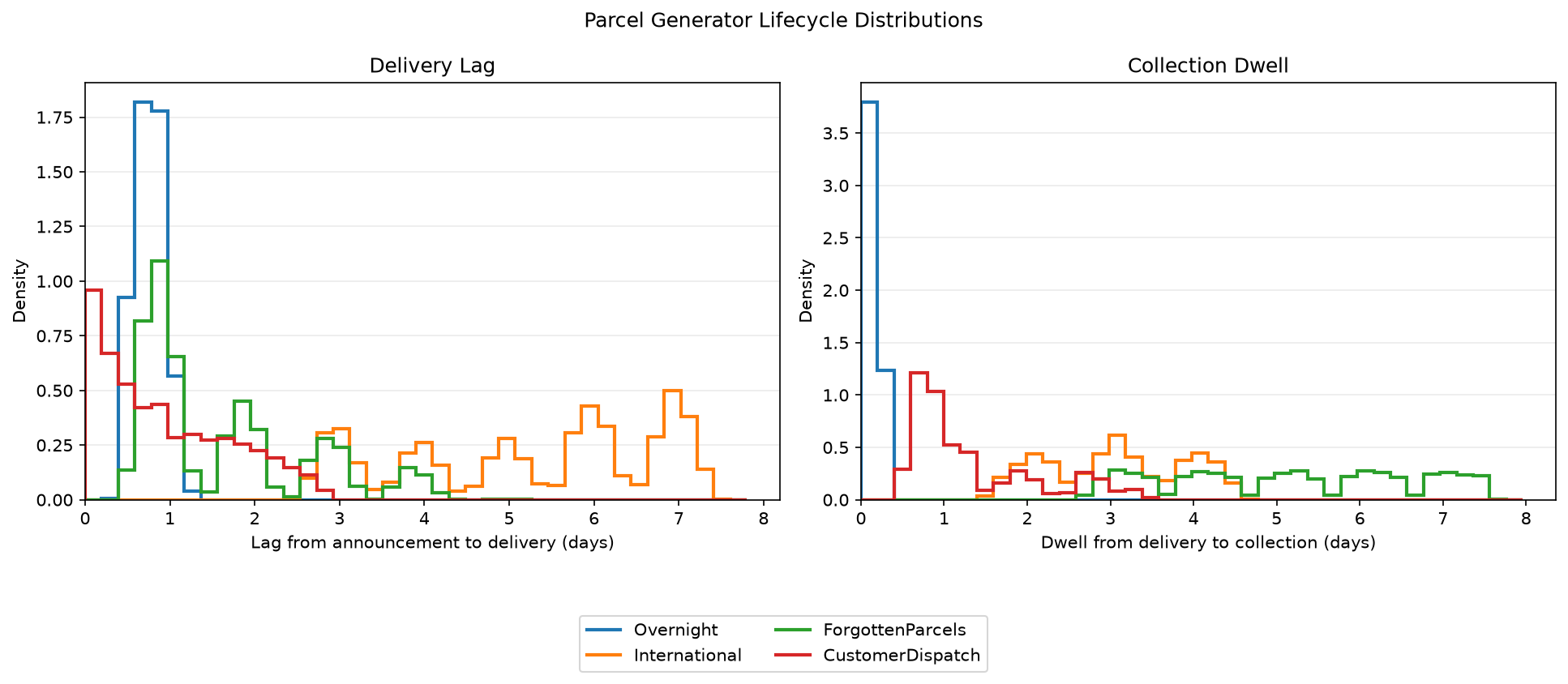
Deliveries always take place on the next calendar day, with 95% occurring in the early morning window between 06:00 and 11:00 and the remaining 5% in a late morning window between 11:00 and 16:00.
Collections happen between 2 to 5 hours after the delivery time, uniformly.
International Parcel Generator
Models international shipments with moderate dwell times and uncertain lag times.
Announcement hours are weighted toward business hours between 8 and 20 o'clock peaking in the morning before lunch and in the afternoon until 17:00. Weekday distribution: Monday at 15%, Tuesday at 25%, Wednesday and Thursday at 20% each, Friday at 15%, and weekends at 5% combined.
Deliveries always occur on a weekday between 8 and 19 o'clock, happening on a randomly selected weekday within 3 to 7 calendar days after announcement.
Collections happen approximately 2 to 4 calendar days after delivery, with the delay sampled from a normal distribution centred at 3 days and std 1 day. Weekday collection hours are biased towards non-business hours of 7 to 9, 11 to 13 or 17 to 21 o'clock, distributed uniformly. Weekend collection hours are uniformly distributed between 9 and 22 o'clock.
Yearly seasonality yields a shift upwards in December, starting in November and ending in January, with slight variations throughout the year.
Forgotten Parcels Generator
Generates regular parcels with respect to delivery pace, which however might remain in the locker for several days.
Announcement and delivery timing follows the standard domestic profile, comparable with Fast or Regular General Purpose Parcel Generator.
Collections occur however three to seven calendar days (uniformly sampled) after delivery, representing a customer who does not promptly retrieve the parcel or might have forgotten about it.
Customer Dispatch Parcel Generator
Generates customer-deposited parcels awaiting courier pickup. Represents an inverse delivery and collection profile.
An announcement reserves a compartment. The delivery event represents the customer depositing the parcel, and the collection event represents a courier pickup on the next weekday during business hours.
Announcements can happen any day 24/7.
Deliveries have a 50% chance of being delivered on the same day of the announcement, 30% chance after 1 days and 20% chance after 2 days. Delivery times though are limited on weekdays between 6 and 9 or 17 to 22 o'clock. Weekend drop-offs happen uniformly between 9 and 22 o'clock.
Collections happen solely between Monday and Friday, during business hours of 9 to 18 o'clock. Collection time, however, strictly happens on the day after the delivery, if the delivery has been done on a weekend, collection rolls over to the next Monday. Mondays therefore represent collection heavy weekdays for this tenant representation.
Rewards and Risk Appetite
The environment deliberately makes acceptance and rejection neutral at decision time, as the policy cannot immediately assess whether an acceptance will ultimately succeed.
The primary learning signal is derived from later operational outcomes, such as whether the parcel has been delivered successfully or not, and how this outcome influences other parcels.
| Event | Reward |
|---|---|
| Accept an announcement | 0.0 |
| Reject an announcement | 0.0 |
| Successful delivery | +1.0 |
| Failed delivery | -5.0 |
| Collection | 0.0 |
The five-to-one outcome asymmetry between a failed and a successful delivery makes capacity failures consequential while still rewarding useful demand.
Roughly speaking, ignoring future interactions, an accepted parcel must have an estimated success probability above 5/6 to be preferable to rejection.
These numbers however are configurable rather than universal truths. Changing them changes the operational meaning of the learned policy.
The reward can also be understood as a risk-appetite parameter. A system that considers failed deliveries extremely costly should use a stronger failure penalty or impose an explicit failure-rate constraint. A system that prioritizes utilization may tolerate more failures in exchange for higher throughput.
An important consideration is that reward alone is not enough to evaluate a policy. A policy could achieve a good reward by rejecting almost everything, avoiding failures but also providing little service. The evaluation therefore needs to report on reliability as well as throughput.
Baselines
Before being able to assess the quality of any policy, we need to establish a baseline to compare against.
Three baselines are designed with deliberately defined characteristics, answering certain questions about different management strategies.
Always Accept Baseline
This baseline accepts every announcement.
Q: What happens if acceptance is maximized without capacity control?
It is not expected to be a strong candidate for capacity management, but it provides an uncontrolled acceptance stress case, showing the consequences of maximizing acceptance without controlling capacity.
It also provides an aggressive point on the throughput-versus-failure tradeoff.
Physical Occupancy Baseline
This policy sees current physical occupancy but ignores accepted pending commitments and future timing. It accepts as long there are physically free compartments.
Q: Is there a need for forecasting elements or does current physical locker state suffice?
Its purpose is to test whether the learned policy gains anything from modelling future timing rather than merely looking at the current number of occupied compartments.
Committed Bookings Baseline
A classic and conservative acceptance strategy. It treats every accepted pending parcel as if it already consumed a compartment. It accepts only if physical occupancy plus pending commitments remains below locker capacity.
Q: What is the cost of never overbooking and staying conservative?
It represents a conservative no-overbooking rule.
It is useful as a reliability-oriented reference point. If the learned policy cannot achieve more throughput at a comparable failure rate, the additional forecasting machinery may not provide practical value.
Observing a Locker
Internally, the environment knows the exact event queue, the announcement, delivery, and collection times of generated parcels, each parcel's lifecycle status, each parcels emitting tenant, physical occupancy as well as accepted pending commitments. The simulator state is therefore designed to be Markovian.
The policy receives only a fixed-size summary, a so called approximate belief state.
Future timestamps, internal source identifiers, and raw calendar information remain hidden. From the policy's perspective, this makes the problem a partially observable Markov decision process, or POMDP.
Observation Space
The policies observation is a high dimensional vector, structured into four conceptual blocks
- Global Locker State describes current occupancy, commitments, and recent outcomes
- Forecast Mean describes expected occupancy at future horizons
- Forecast Failure Risk describes the probability of reaching capacity at those horizons
- Candidate Fingerprint and Comparison Features describe the parcel under consideration and its relationship to future locker pressure
The observation space is intentionally designed to exclude any direct information about the parcel's tenant or calendar features such as day of the week, hour of the day, or time of the year.
This ensures that a trained policy can adapt to various tenants and changing patterns. The policy should only have access to the historical delivery and collection patterns of a parcel, not the identity of the tenant or the specific time of the announcement.
Global Locker State
This block captures the locker’s current status and recent performance:
- Physical Occupancy Ratio: Current compartments in use relative to capacity.
- Pending Commitments Ratio: Accepted but undelivered parcels relative to capacity.
- Total In-Flight Parcels: Sum of physical occupancy and pending commitments, normalized by capacity.
- Recent Rejection Rate: Fraction of recent parcels rejected.
- Recent Delivery-Failure Rate: Fraction of recent deliveries that failed due to full lockers.
These metrics summarize the locker’s state without exposing raw event histories.
Forecast Mean
The expected normalized occupancy (i.e., average compartment usage) is computed for 11 future horizons:
$$1, 2, 4, 8, 16, 24, 36, 48, 72, 120, 168 \text{ hours}$$
For each horizon $u$, the forecast aggregates the occupancy probabilities of all active parcels:
$$\mu(u) = \frac{1}{C} \sum_{i=1}^{n} p_i(u),$$
where $C$ is the locker capacity, and $p_i(u)$ is the probability that parcel $i$ occupies a compartment at time $u$.
- For delivered parcels, $p_i(u)$ is the conditional survival probability that the parcel remains uncollected by $u$, given it has not been collected yet.
- For pending parcels, $p_i(u)$ accounts for both the probability of delivery by $u$ and the subsequent dwell time.
The forecast mean can exceed one when accepted commitments imply expected overbooking. A value of 1.0 means expected occupancy equals physical capacity; it does not mean that the locker is guaranteed to be full.
This block helps the policy anticipate congestion trends.
Forecast Failure Risk
While the mean forecast provides average occupancy, this block estimates the probability of overflow (i.e., $N(u) \geq C$) at each horizon.
Here, $N(u) = \sum_{i=1}^{n} X_i(u)$, where $X_i(u)$ is a Bernoulli variable indicating whether parcel $i$ occupies a compartment at $u$.
Under the assumption of conditional independence, $N(u)$ follows a Poisson-binomial distribution, and the failure risk is:
$$R(u) = P(N(u) \geq C) = \sum_{r=C}^{n} q^{(n)}_r(u),$$
where $q^{(n)}_r(u)$ is the probability that exactly $r$ parcels occupy the locker at $u$.
This exposes tail risk: even if mean occupancy is moderate, a high $R(u)$ signals a significant chance of overflow.
Candidate Fingerprint and Comparisons
The current candidate cannot be added directly to the aggregate forecast because the policy is deciding whether to accept it. Instead, the environment provides a compact candidate-risk comparison feature.
Let $t_a$ denote a parcels announcement time, $t_d$ denote a parcels delivery time and $t_c$ denote a parcels collection time, we define
- Lag Quantiles: Empirical quantiles ($q \in \{0.10, 0.25, 0.50, 0.75, 0.90\}$) of the delivery lag $L = t_d - t_a$ (Stored as $\log(1 + h)$ space to handle skew).
- To assess the distribution of delivery times, from typical p50 to worst-case p90.
- Dwell Quantiles: Similarly, quantiles of the collection dwell $D = t_c - t_d$.
- Lag Confidence: $c(n) = 1 - \exp(-n/20)$, where $n$ is the number of lag samples for the parcel’s context.
- To distinguish reliable patterns (high $n$) from uncertain estimates (low $n$).
- Dwell Confidence: Analogous to lag confidence.
- Historical Delivery Success Rate: Historical success probability for the parcel’s source tenant.
- Candidate Delivery-Time Congestion Risk: Interpolated failure risk $\widetilde{R}(\ell_j)$ at the candidate’s likely delivery times $\ell_j$, weighted by their probabilities.
- To estimate the risk of locker overflow if the candidate is accepted, without circularly including it in the aggregate forecast.
- Lag Uncertainty: $U_{\text{lag}} = q_{0.90}(\log(1+L)) - q_{0.50}(\log(1+L))$, measuring the spread between the median and 90th percentile lag.
- To identify parcels with highly variable delivery times, which may pose higher planning risk.
This block enables the policy to assess the candidate’s timing and risk in the context of the locker’s likely future state.
Behavioural Profile Modeling
The observations are derived from a rolling behavioural profile tracker for each parcel source, it measures
- Delivery Lag Samples (how long after announcement delivery typically occurs)
- Collection Dwell Samples (how long parcels occupy compartments)
- Delivery Success/Failure Outcomes
conditioned on day of week and time-of-day buckets (night, morning, midday, afternoon, evening).
The behavioural profile tracker allows configuration of the historical data retention period. By default, it considers locker activity from the past 21 days, with fallback delivery and collection profiles available to address cold-start scenarios.
Training a Policy
Proximal Policy Optimization (PPO) was chosen as a well-established actor-critic algorithm that supports discrete actions and provides stable policy updates through a clipped objective. Its policy estimates the probability of each action, while a value function estimates the expected future reward. This combination is useful for the delayed rewards and partial observability present in the locker environment.
PPO is trained on a matrix of 9 different pressure level and locker size configurations with a budget of 500.000 timesteps each.
| Pressure Levels | Locker Sizes |
|---|---|
| 0.4 | 10 |
| 0.7 | 50 |
| 1.0 | 80 |
This means the training procedure yields 9 independent policies trained on 1 pressure/locker-size combination of the Cartesian product of three pressure levels and three locker sizes.
A pressure level dictates the number of parcel announcements generated over a one-year simulation period, it's a dimensionless metric that scales with locker size to ensure comparability across lockers of varying capacities. Formally, the total number of announcements $N$ is given by:
$$N = \text{pressure} \times \text{locker\_size} \times 365$$
- $\text{pressure}$ is a normalized demand intensity parameter, representing the average number of parcel announcements per compartment per day.
- $\text{locker\_size}$ is the number of compartments in the locker.
A locker of size 50 confronted with a pressure level of 0.7 therefore needs to decide on 12775 parcels throughout the simulated year.
Generator distributions are fixed depicting a challenging but realistic smart locker scenario. Shifts in tenant distributions apart from those already modeled within generator implementations are deferred for dedicated evaluation on policy distribution shift generalization, therefore the training generator distribution does not contain the full spectrum of available generators.
| Tenant | Distribution |
|---|---|
| Fast General Purpose | 80% |
| Overnight Shipping | 10% |
| International Shipping | 10% |
Episode simulations are started within a uniformly random picked point in time throughout the year and end roughly after 365 days (pending deliveries and collections after the last policy decision are still processed)
Checkpoints are saved every 10,000 environment timesteps. For each pressure/locker-size combination, the checkpoint with the highest mean validation reward across five independent episodes is selected for reporting and evaluation.
Training Results
The training behaviour seems to be consistent with policy learning to trade acceptance against future delivery risk.
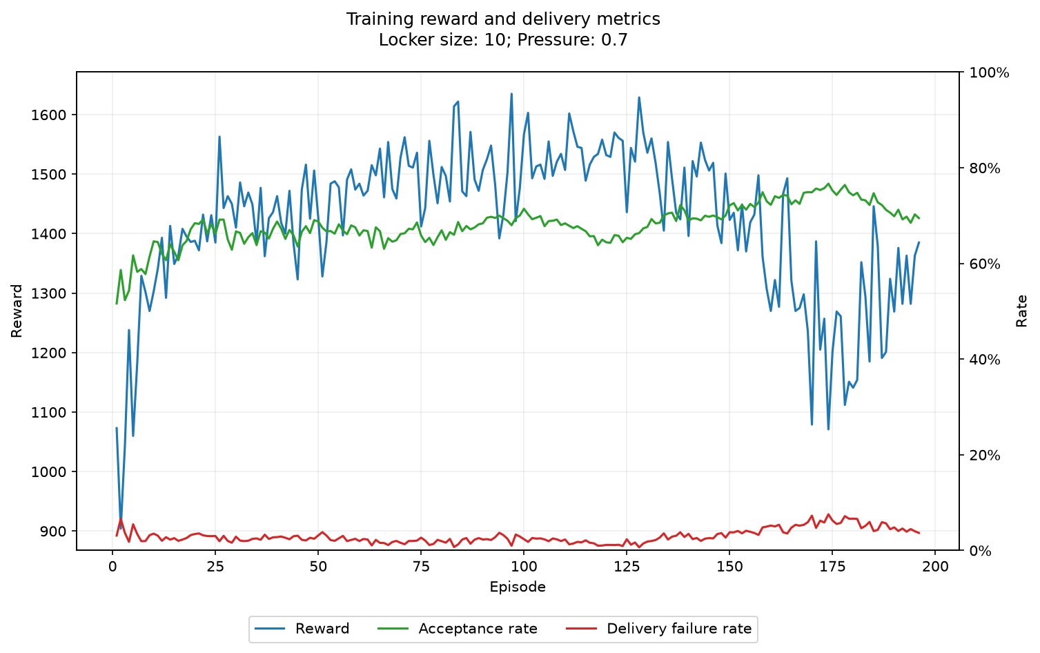
Notably, all policies stayed rather conservative, with respect to delivery failures, as delivery failures are penalized heavily due to the five-to-one ratio, which makes the policy considerate on the acceptance of new parcels.
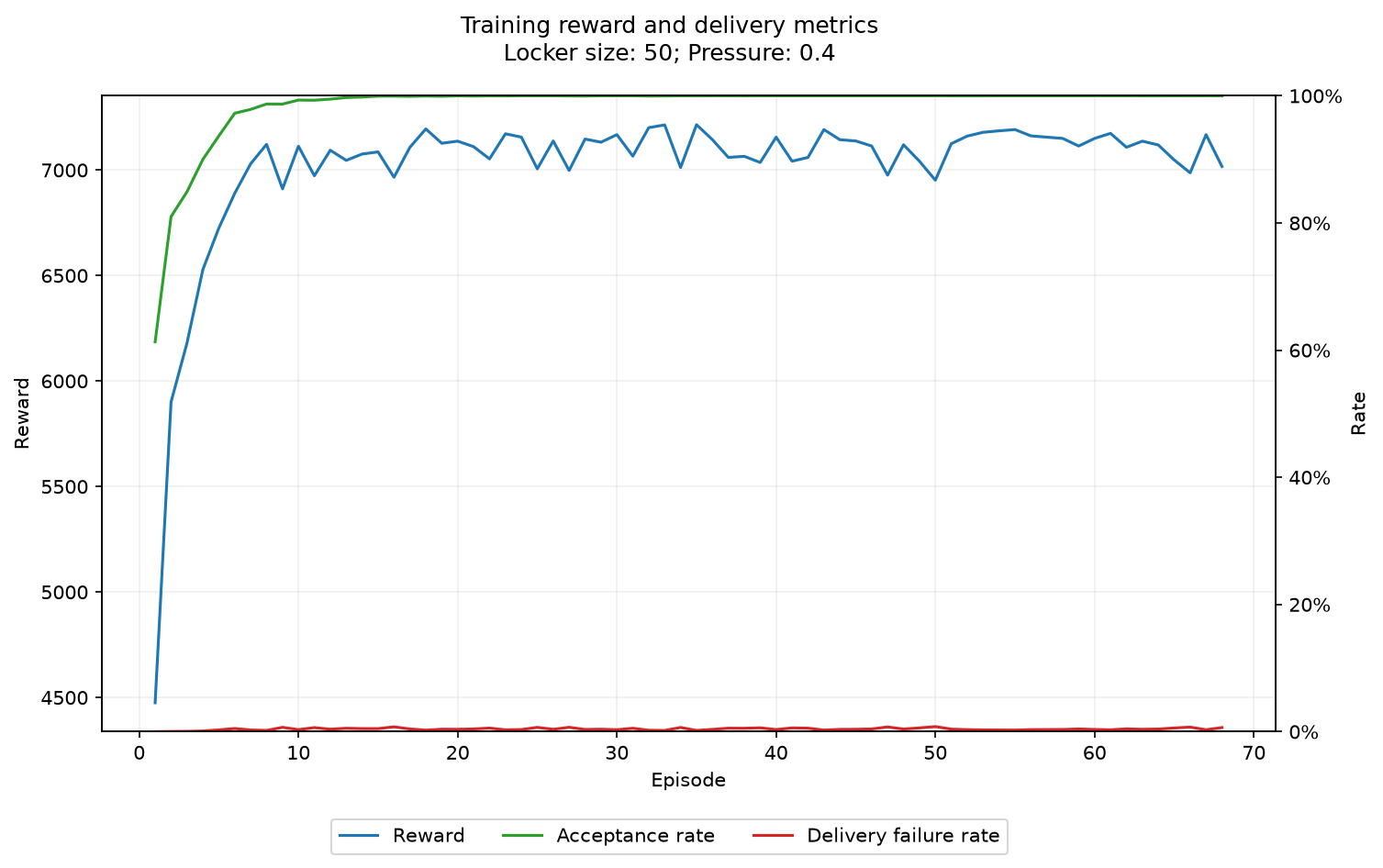
Policies confronted with pressure level 0.4 seem to have learned that the overall locker pressure is low enough that it allows to accept close to every parcel without incurring delivery failures and in turn reward penalties. It's up for evaluation to see if these policies have learned anything useful in terms of effective capacity management.
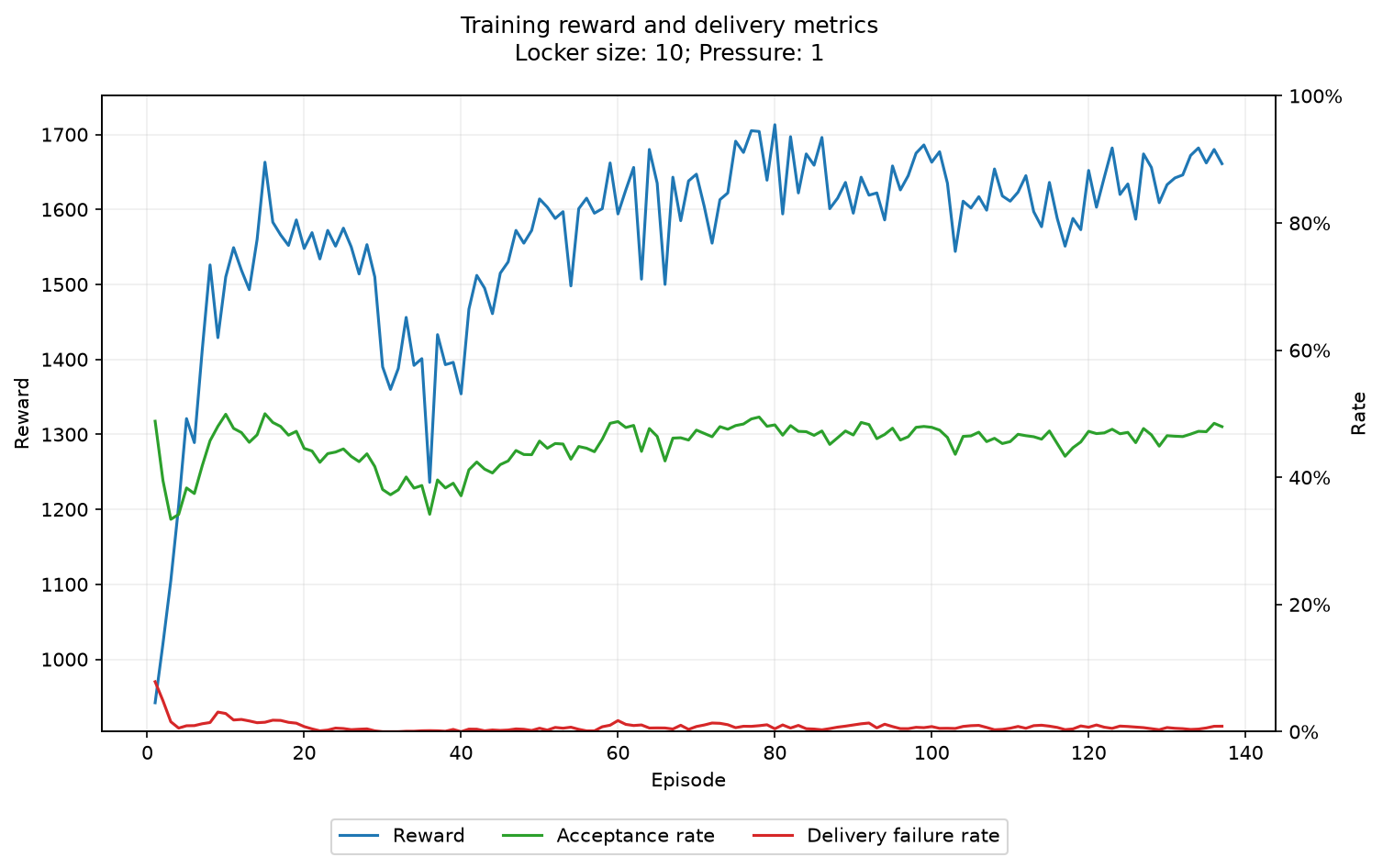
On the contrary, policies tasked to handle pressure level 1.0 manage to keep the delivery failure rate similarly low, however need to be more selective with respect to parcels to accept or reject. So much so as that locker pressure 1.0 policies tend to accept only 50% or above of the announced parcels. It remains to be seen if this strategy is too conservative for capacity management by comparing to baselines later on.
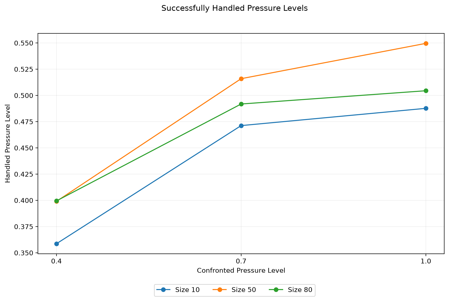
Telling by the successfully handled volume, the trained policies seem able to handle between 0.35 to 0.55 pressure, notably increasing with the confronted pressure level. Intuitively this does make sense, a higher pressure level yields more opportunities for "smarter" overbooking, whilst it also necessitates careful selection of parcels to be accepted.
At higher pressure levels however the handled pressure level seems to flatten out at some point, indicating saturation of the policies capabilities on capacity management.
| Accepted parcels (% of announcements) | Pressure 0.4 | Pressure 0.7 | Pressure 1.0 |
|---|---|---|---|
| Size 10 | 1320 (90%) | 1737 (68%) | 1795 (49%) |
| Size 50 | 7300 (100%) | 9560 (75%) | 10288 (56%) |
| Size 80 | 11680 (100%) | 14449 (71%) | 14935 (51%) |
For each locker size, the acceptance rate decreases as pressure increases, indicating more selective behaviour under higher demand.
In general, delivery failure rate amongst the trained models is between ~0.1 % up to ~2.5 %. Depending on the acceptable delivery failure rate, the reward might be tweaked such that it either penalizes failed deliveries harsher or less harsh.
Evaluating the Policy
Training curves show that optimization occurred, but not whether the learned policy generalizes. We therefore freeze the selected policies and evaluate them without exploration on independent episodes using the same generated scenarios and random seeds for every policy across every baseline.
Generator distributions in these evaluations are equal to the training distribution, while the episodes are new independently sampled. Dedicated evaluations on unseen generator distribution generalization, apart from those already modeled within the generator implementations, are deferred to their own section.
Each policy has been trained on a specific configuration combination of locker size and pressure level. However, as the policies need to perform well across all pressure levels, we opt to showcase evaluations of pressure levels throughout 0.2, 0.4, 0.6, 0.8 and 1.0.
Baselines
As a first step we evaluate the trained policies compared to the baselines on locker sizes the policies have been trained on, across all pressure levels.
Delivery failure rate is shown as a dashed line, referencing the right y-axis.
Comparing them against the classic but conservative Committed Bookings Baseline, the trained policies clearly outperform in terms of throughput, while keeping delivery failure rate comparably low.
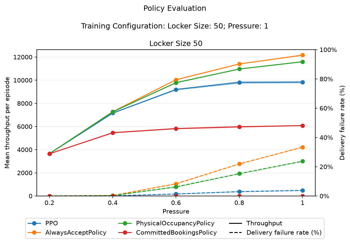
When comparing against the less risk-averse Physical Occupancy Baseline we can see that the trained policy indeed seemingly cultivated some kind of planning behaviour.
Throughput is often comparable to Physical Occupancy Baseline or slightly below, at the benefit of a much lower delivery failure rate. This indicates that the sole information of the current locker state is not sufficient information to perform qualitative capacity management.
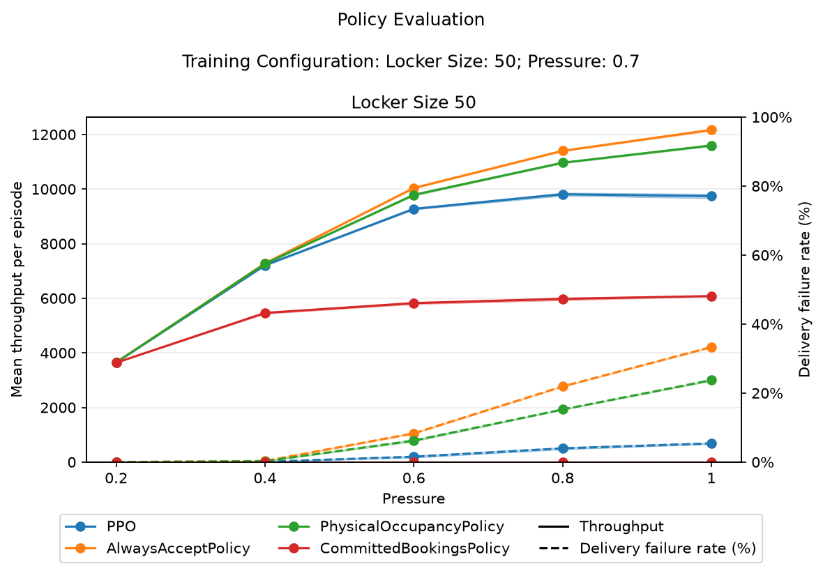
Pressure Levels
As lockers get bigger, uncertainty increases as more and more parcels need to be managed and considered when calculating forecast capacity and delivery failure risks. This can be seen at locker size 80 clearly.
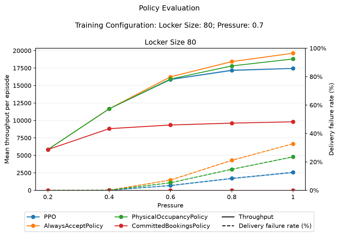
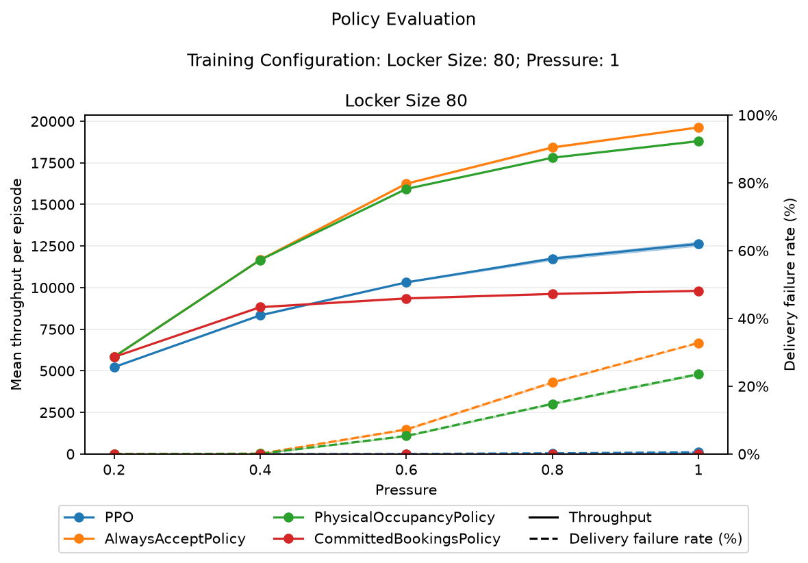
Locker Size 80, Pressure Levels 0.7 and 1.0 evaluated against baselines on all pressure levels
A policy trained on pressure level 1 performs well in terms of delivery failure rate, but suffers from a slight damp in throughput at lower pressure levels. It's still performing better or equal to the Committed Bookings Baseline, especially at higher pressure levels, but does not manage closely hug the Physical Occupancy Baseline as tightly as before.
A policy trained on a locker of size 80 and a lesser pressure level of 0.7, hugs Physical Occupancy Baseline tighter again, but at the cost of noticeably elevated delivery failure rate when being evaluated on pressure level 1.0. It seems as uncertainty increases with locker size, the more important it becomes to train a policy on high pressure levels, at the cost of it becoming conservative in situations it wouldn't need to be as conservative.
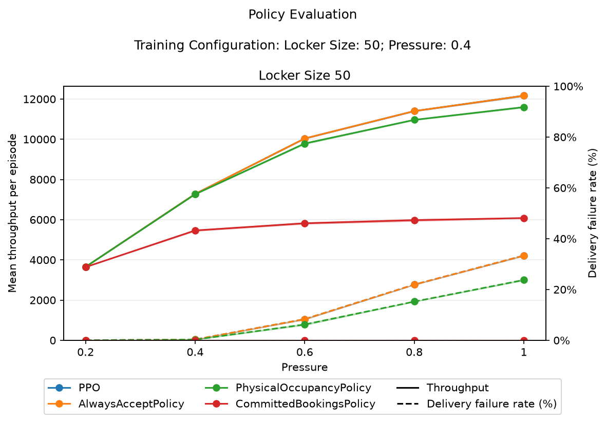
In 2 out of 3 cases, a policy trained on pressure level 0.4 didn't learn anything useful, and opted for an always accept strategy, mimicking the Always Accept Baseline. It seems reasonable to argue that policies need to experience some level of pressure in order to be forced to learn a useful policy.
In general the standard deviation of the trained policies stays small, which indicates confidence in the learned behaviour.
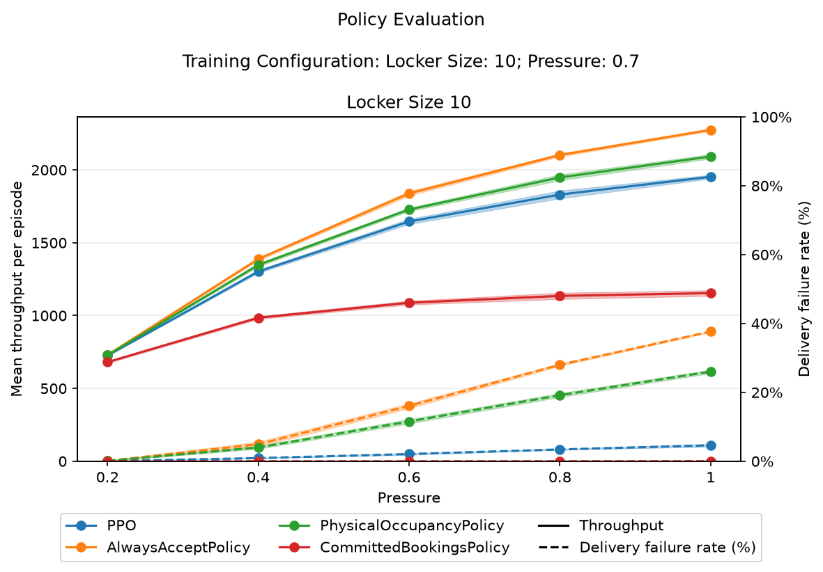
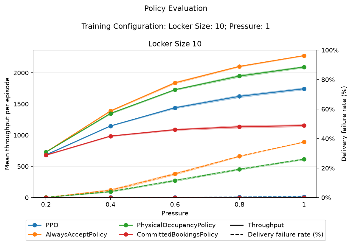
Locker Size 80, Pressure Levels 0.7 and 1.0 evaluated against baselines on all pressure levels
Generally speaking, it can be observed that training a policy at a higher pressure level does not necessarily render it ineffective for application in lower pressure scenarios. On the contrary, the majority of such policies demonstrate strong performance across the entire spectrum of pressure levels.
However, training at higher pressure levels, while unlocking more optimization strategies, also seemingly makes the policy more conservative overall.
Locker Sizes
Having evaluated policy performance on trained locker sizes and pressure levels, we now test cross-size generalization.
This means we evaluate whether a policy trained on one locker size retains effectiveness on unseen locker sizes. This assesses robustness and adaptability, with throughput and delivery failure rate again evaluated across all pressure levels.
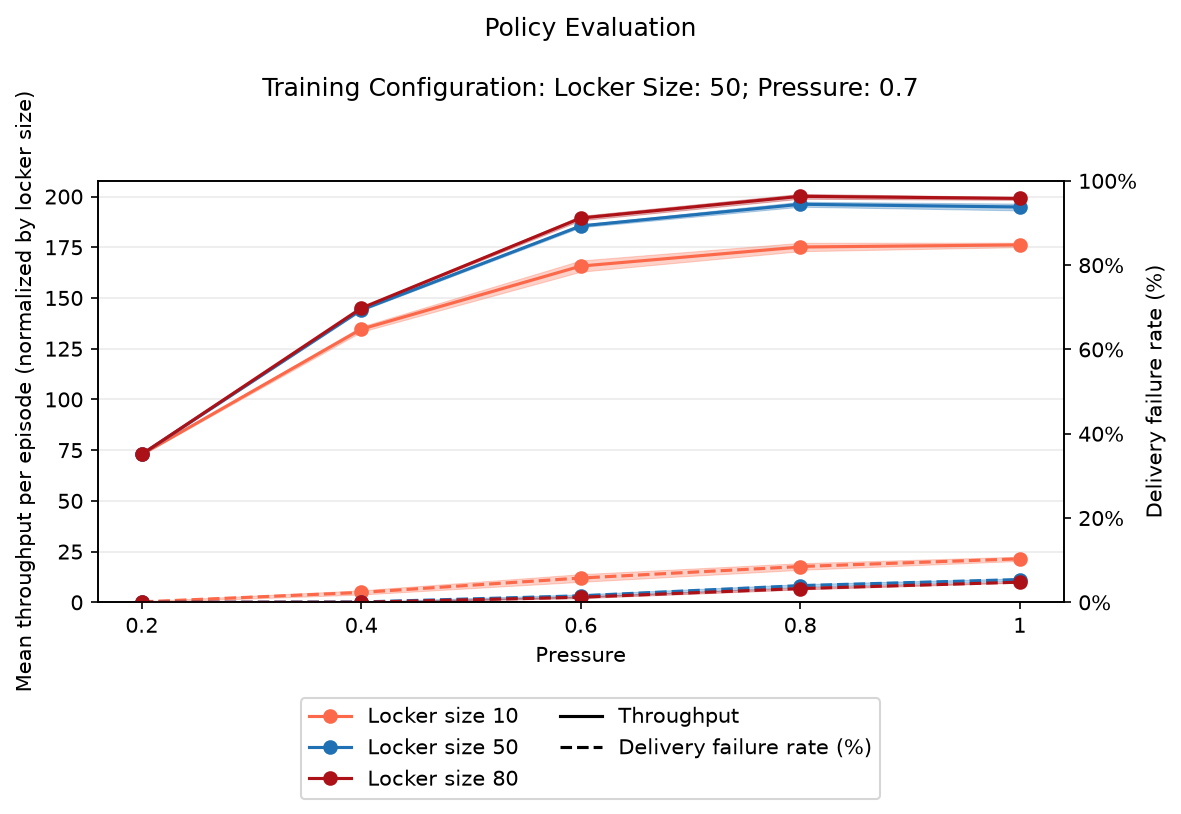
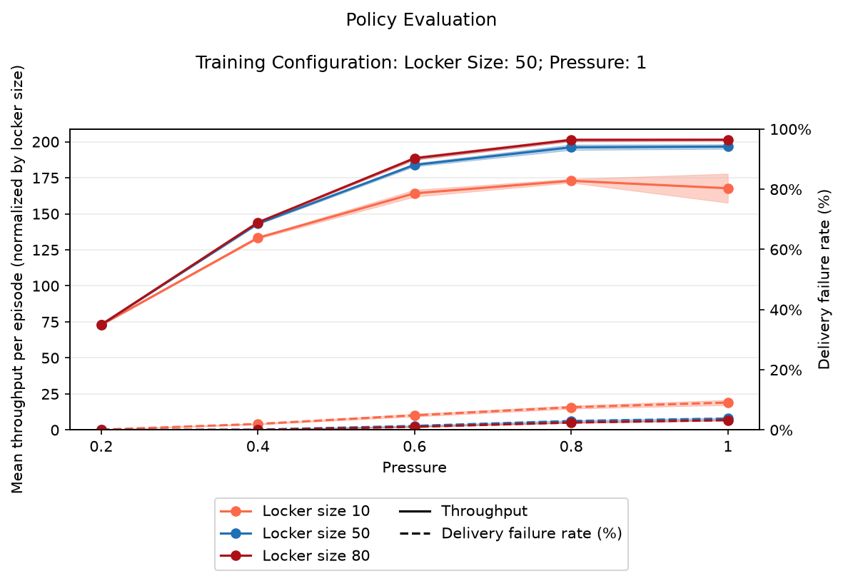
Policies trained on locker size 50 and pressure level 0.7 respectively 1.0 evaluated on their transferability to different locker sizes across all pressure levels
Most often, the policies seem to be well transferable across locker sizes retaining their overall efficiency, which is especially visible for the interchangeability of policies trained on lockers of size 50 and 80.
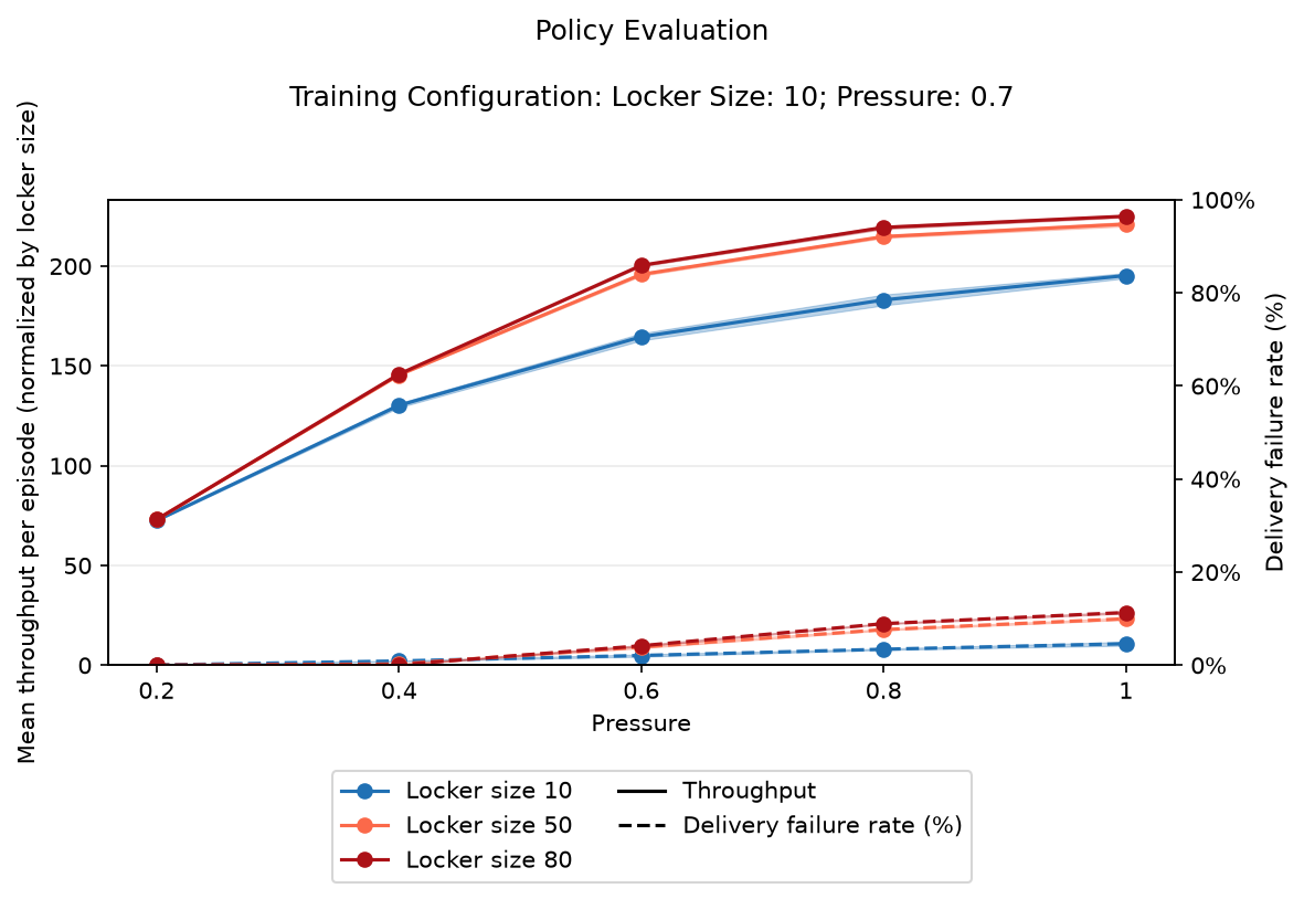
However, policies trained on too small lockers sizes, such as those trained on locker size 10, seem to have problems scaling up to larger locker sizes 50 and 80.
The contrary seems to be true as well, although not as pronounced, policies trained on higher locker sizes 50 and 80 seem to also experience slight performance degradation when managing lockers of size 10.
This might be due to the changed precision of certain observation features relative to locker size and locker utilization, when transferring across locker sizes.
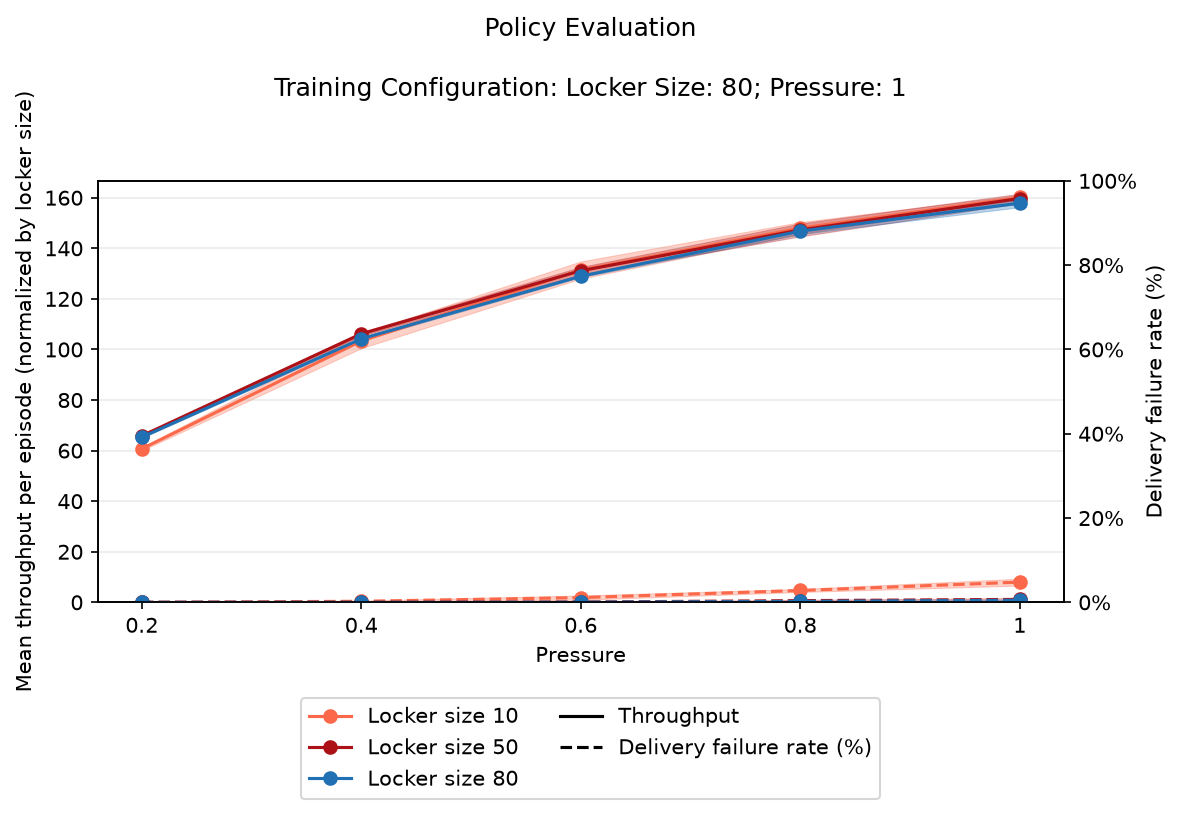
Arguably a transfer can be done as long as it's not an extreme case.
It's though debatable if one might be safer off training dedicated policies for dedicated locker sizes to achieve maximum and better predictable performance in terms of high throughput and low delivery failure rate. After all locker sizes do not change as often as pressure varies.
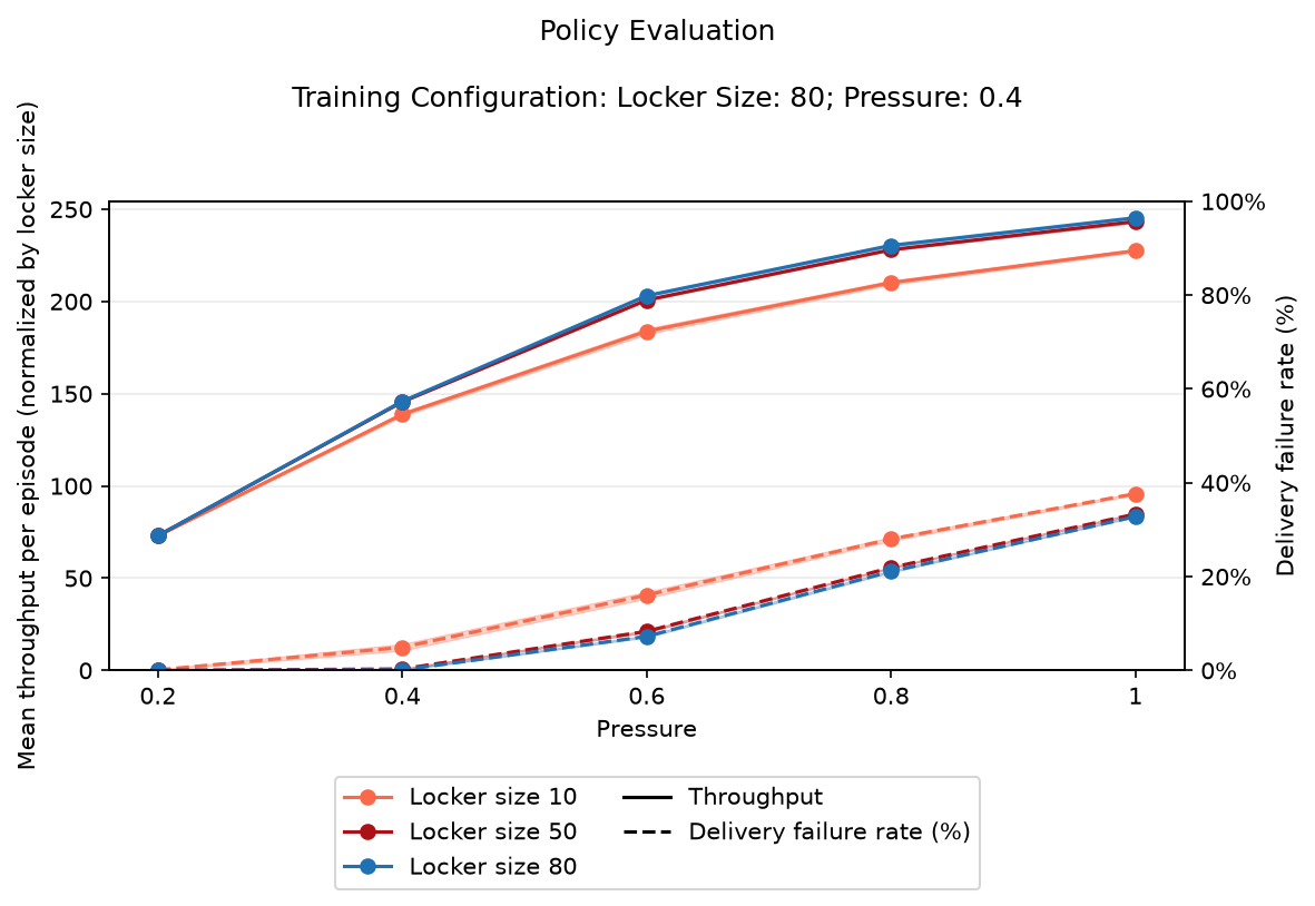
Also in this comparison scenario we can clearly see that policies trained on pressure levels such as 0.4, which are not challenging enough for the policy to learn any useful capacity management strategies, bad results only worsen when transferring them.
Looking Deeper: Tracing an Episode
To get a better understanding of the policy behaviour, we trace the decisions of the model throughout one episode along with the decisions of the baselines to compare with, which all operate on an equally seeded environments for 1:1 comparability.
As we've established before, cross-size transfer is possible for some cases, and increased/decreased pressure levels can also be handled well in most scenarios.
However, in this section, policies are investigated on episode configurations of locker size and pressure level they've been trained on in order to get an accurate picture of the trained behaviour, not the generalized/transferred behaviour.
Cumulative Delivery Successes and Failures
We analyze cumulative delivery successes over a one-year episodic period, benchmarking them against baseline performance. To assess behaviour, outcome, and variation throughout the episode, we visualize cumulative successes, delivery failure rates, and rejection decision rate.
We are able to observe a similar picture as we did beforehand when analyzing the summary statistic evaluations, however we notice that the trained policy as well as the baselines seem to calibrate at the beginning of an episode.
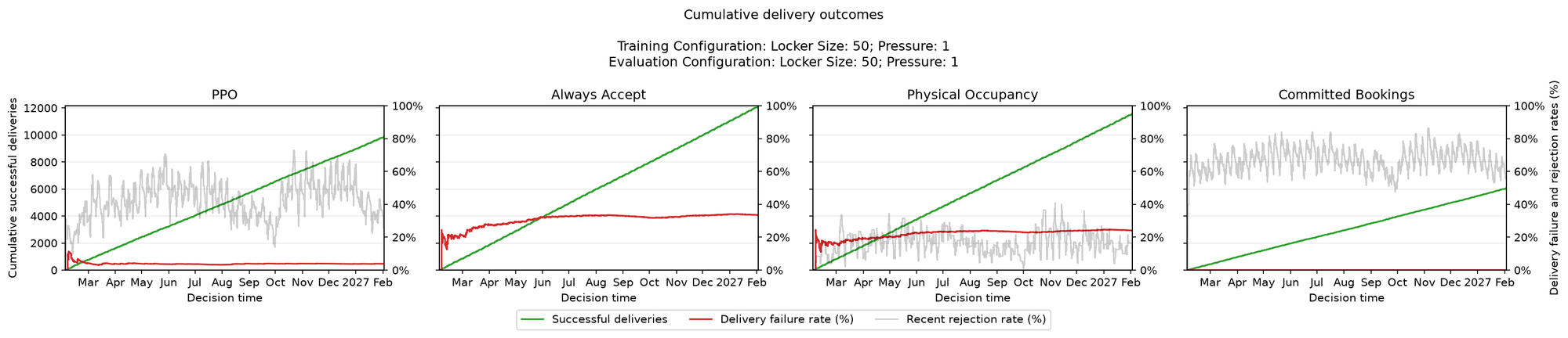
The trained policy retains only 21 days of history to build the behaviour profile as well as forecast metrics, hence slight fluctuations at the beginning are expected as a cold-start calibration. Throughout the episode then, the trained policy maintains a steadily low delivery failure rate compared to the baselines.
Successful deliveries are again close to the Physical Occupancy Baseline, whilst keeping failure rate considerably lower than the baseline.
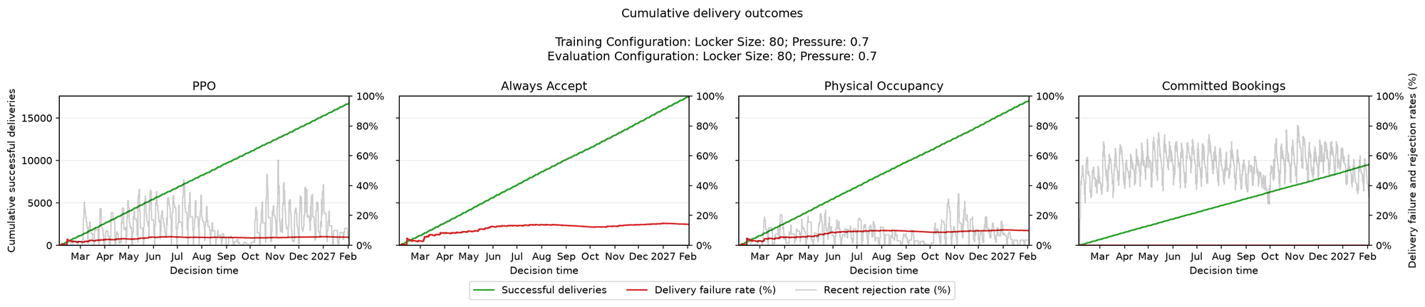
Rejections also seem to be in a sweet-spot between the Physical Occupancy Baseline and the Committed Bookings Baseline.
While the Committed Bookings Baseline rejects considerably more parcels compared to the Always Accept Baseline, it achieves only an episode-end throughput of roughly 50% to 60% relative to the Always Accept Baseline.
The trained policy, however, manages to successfully deliver between roughly 90% and 95% relative to the Always Accept Baseline, while only rejecting slightly more parcels than the Physical Occupancy Baseline, at a significantly lower delivery failure rate compared to both.
Locker Utilization and Occupancy
In addition to cumulative delivery successes, failure rates and rejection decision rates, we also monitor the utilization and occupancy of the locker throughout the episode.
We distinguish between physical occupancy, referring to parcels which have been successfully delivered, and pending commitments, which at the time of the decision have not been delivered yet, the policy, or baseline however has already accepted.
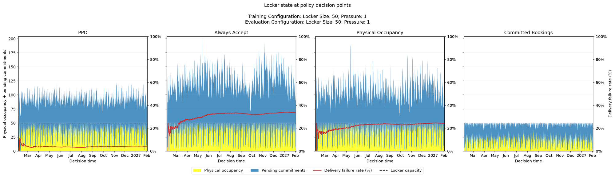
As expected, the Committed Bookings Baseline never exceeds the nominal locker capacity, visibly underutilizing compartment space due to its inefficient capacity management strategy.
In contrast, the trained policy strikes a balance: its physical occupancy typically surpasses that of the Committed Bookings Policy while remaining slightly below the more aggressive Always Accept Baseline and Physical Occupancy Baseline.
However, depending on demanded pressure, it optimizes both available space and pending commitments, achieving a 150% utilization rate peaking at 200% during periods of low physical occupancy.
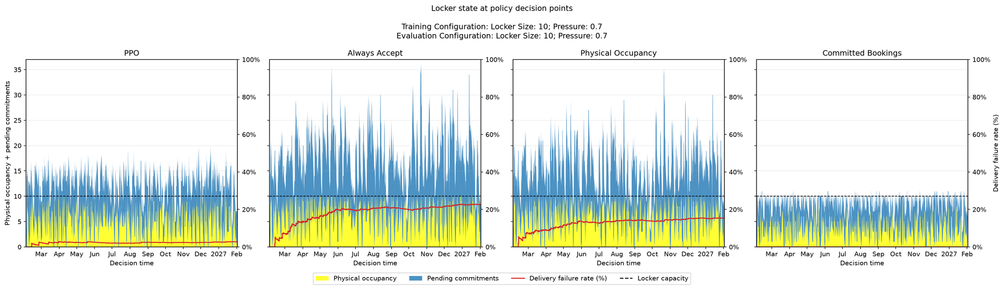
The periods of low physical occupancy are likely weekends, as within the utilized generator setup only the Overnight Shipping tenant does deliver over the weekend, while the others delivery only on weekdays, with collections happening throughout the week.
Tenant Acceptance
Finally, we examine whether certain policies, baselines, or delivery profiles disproportionately benefit some tenants over others under specific conditions.
Yet, it may still implicitly favor certain tenant profiles.
To address fairness, fairness proxies should be included in the observation space, and a fairness metric should be integrated into the reward function as learning signal.
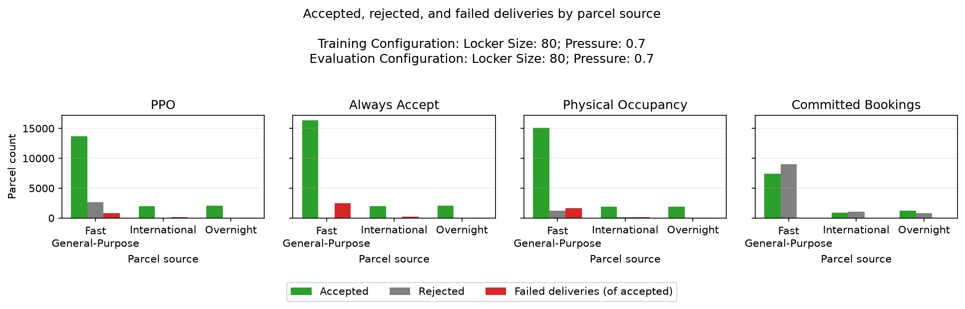
We evaluate acceptance, rejection and failed deliveries by parcel source for the policy as well as the baselines to compare with.
Verification of rejections from the Committed Bookings Baseline and the Physical Occupancy Baseline suggests that no tenant is inherently favoured or disadvantaged in terms of acceptances or rejections based on their delivery and collection profile.
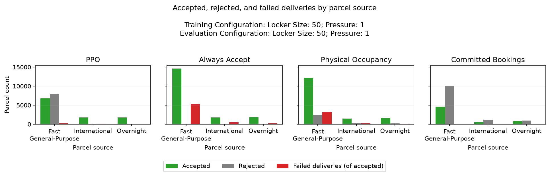
On this occasion however, it is notable that in the high pressure scenario depicted, the policy seems to have favoured parcels of International Shipping and Overnight Shipping, as it rejected close to none of these tenants parcels. Whereas the bulk of rejections falls on the more general default parcel provider.
It might be less pronounced than the high pressure scenario, but also in the 0.7 pressure level plot we can see a tendency for this behaviour.
This observation may seem counterintuitive, as Overnight Shipping parcels require rapid accommodation, while International Shipping parcels present challenges due to high uncertainty, long delivery lag times, and extended dwell periods.
One might however reason that:
- Fast General Purpose Tenant Parcels, comprising the majority of demand, typically arrive within 1 to 2 days and occupy locker space for roughly another day. Under high pressure, they are the primary source of near-term congestion.
- Overnight tenant parcels, while arriving promptly, have a minimal occupancy footprint, as they remain in the locker for only 2 to 5 hours.
- International tenant parcels arrive after a longer delay of 3 to 7 days, allowing existing parcels to clear before their delivery. Although they have longer dwell times, they account for just a minority of the demand, and their deliveries are distributed over time.
This seems also plausible when looking at the results of the Always Accept Baseline, Default tenant parcels seem to have the highest failure rate, consequently, triaging them most allows for throughput optimizations, while Overnight parcels result in fewest failures.
Generator Distribution
In addition to assessing the trained policies under varying pressure levels and unseen locker sizes, we further evaluate their robustness by testing them on a different, previously unseen tenant distribution. This allows us to compare their performance against the baseline methods under yet another new condition.
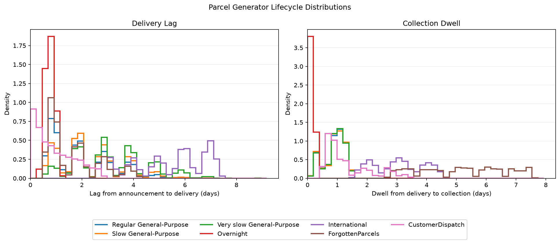
We evaluate the policies on a challenging yet plausible unseen tenant distribution. To this end, we replace the Fast General Purpose tenant with three distinct tenants, while retaining Overnight and International tenants, and adding Forgotten Parcels and Customer Dispatch generators.
| Generator / Tenant | Original Distribution | Unseen Distribution |
|---|---|---|
| Fast General Purpose | 80% | - |
| Regular General Purpose | - | 20% |
| Slow General Purpose | - | 20% |
| Very Slow General Purpose | - | 20% |
| Overnight | 10% | 10% |
| International | 10% | 10% |
| Forgotten Parcels | - | 5% |
| Customer Dispatch | - | 15% |
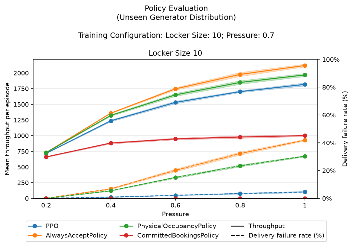
In general the trained polices seem to hold up well even on unseen tenant distributions. We see slightly reduced throughput compared to the evaluations on the original distribution.
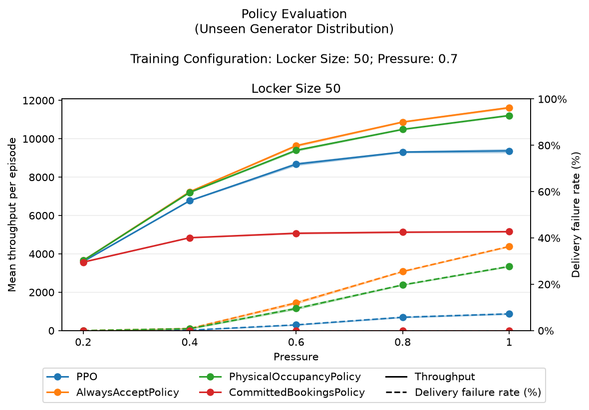
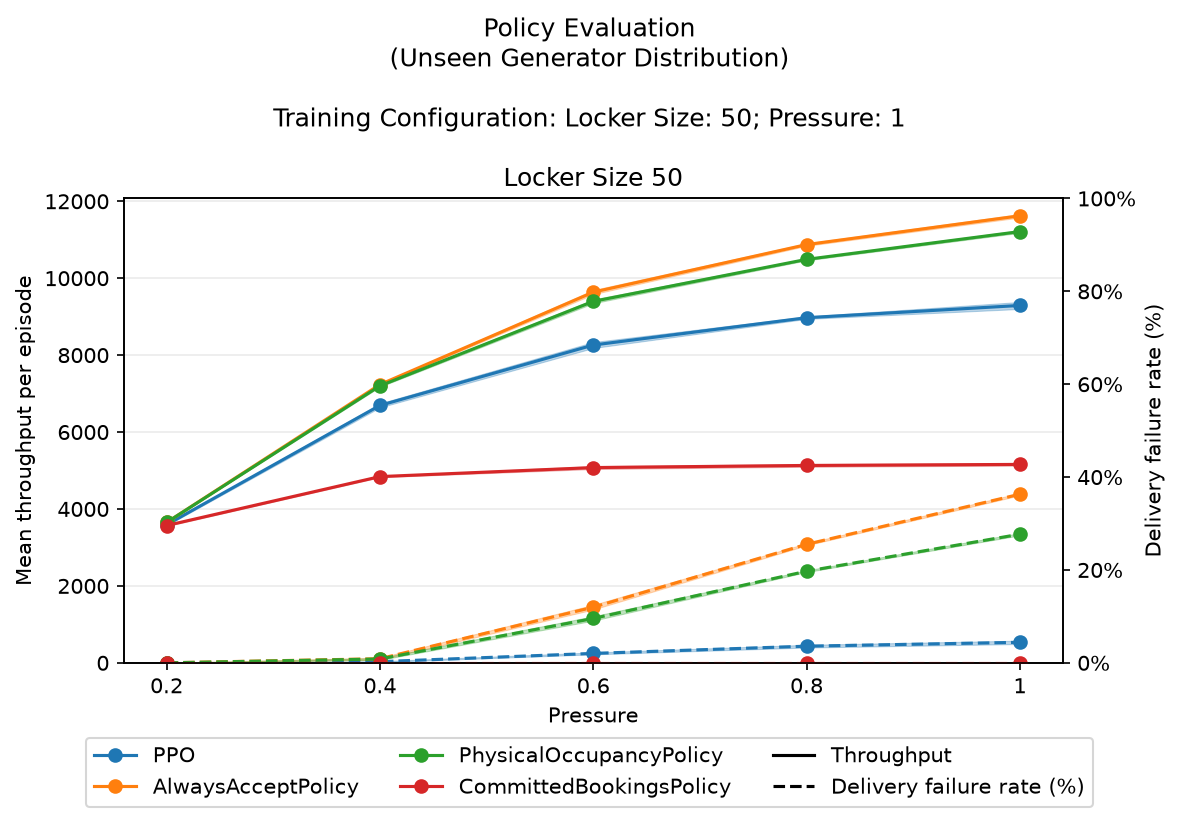
Locker Size 50, Pressure Levels 0.7 and 1.0 policies evaluated against baselines on all pressure levels on previously unseen generator distribution
As before, locker size transfers work well between sizes 50 and 80. However, here even more pronounced, transferring a policy trained on size 50 to handle size 10 yields high variance in the results. Although the delivery failure rate stays remarkably low, throughput is visibly reduced and exhibits high variance at high pressure levels.
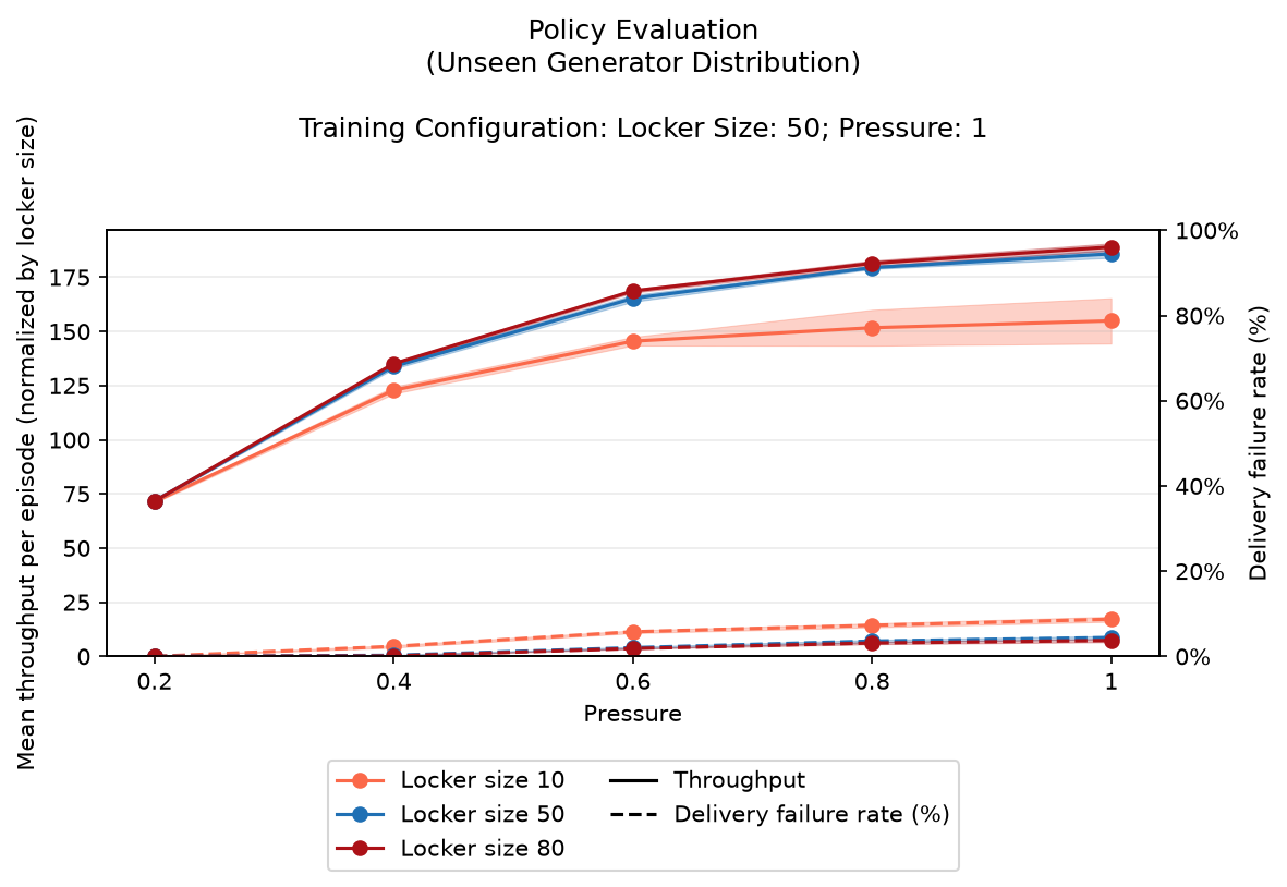
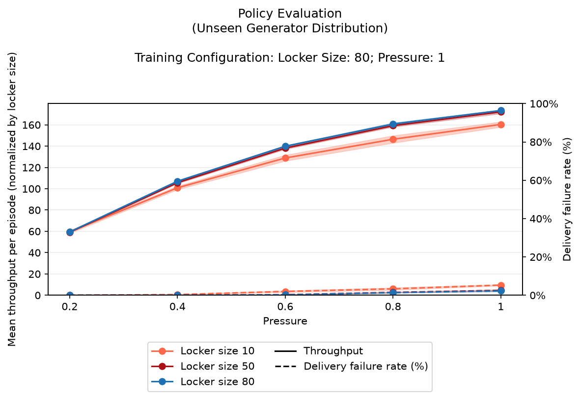
Policies trained on locker size 50 and 80, pressure level 1.0 evaluated on their transferability to different locker sizes across all pressure levels on previously unseen generator distribution
Similarly, as discussed in the previous sections, although policies trained on higher pressure levels tend to be more conservative overall, their transferability is increased, likely due to the more conservative nature instilled in them.
The policy trained on locker size 80 with a higher pressure level transfers well to this new and unseen tenant distribution.
In contrast, the policy trained at a pressure level of 0.7 struggles to adapt to the new tenant distribution, resulting in a higher delivery failure rate. However, this policy instance (Locker Size 80; Pressure 0.7) also showed elevated failure rates in evaluations with the original tenant distribution. Thus, it may simply be a suboptimal policy.
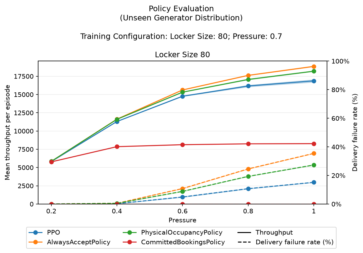
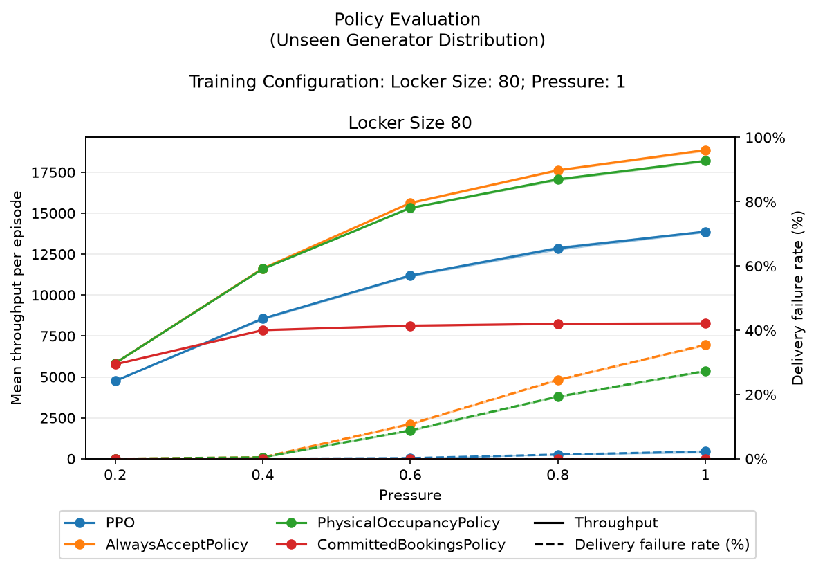
Locker Size 80, Pressure Levels 0.7 and 1.0 policies evaluated against baselines on all pressure levels on previously unseen generator distribution
Apart from this single instance the policies generally perform well. The results show only minor changes in overall performance, even in challenging evaluation scenarios involving unknown tenant distributions, locker size transfers, and varying pressure levels.
Challenges and Unsuccessful Approaches
In this section, we discuss the strategies that did not yield the expected results, along with the reasoning behind their failure.
Biased Reward Shaping
Initially, there was an intuitive (though premature) inclination to adjust the reward signal to explicitly incentivize acceptance decisions or penalize rejections. However, this approach lacked a strong theoretical foundation and was driven more by intuition than rationale.
- Rewarding acceptance decisions introduced unnecessary bias into the learning process. As previously established, the benefits of accepting or rejecting a parcel cannot be determined prematurely.
- In some cases, the model began mimicking the "accept all" baseline, as the cumulative reward for accepting many parcels outweighed the penalties from rejections, leading to suboptimal behaviour.
The reward structure was revised to depend solely on the outcome of decisions rather than the decisions themselves, using the five-to-one ratio presented above. While this initially seemed harder for the policy to learn, it ultimately resulted in more stable training and better long-term performance.
Variable Locker Size Training
Another approach involved training a single policy on environments with varying locker sizes. Although the environment still retains some remnants of this design (e.g., locker-size independent pressure level definition and locker size information in the observation space), the method introduced significant challenges.
- Different locker sizes led to varying episode lengths (in terms of decisions), which increased variability in training.
- Attempts to mitigate this by capping the maximum number of decisions per episode (e.g., 2000) created new problems:
- For small lockers (e.g., size 10), 2000 decisions might cover most of the year’s parcel announcements (e.g., 3650 at pressure level 1.0).
- For large lockers (e.g., size 50), 2000 decisions represent only a small fraction of the total (e.g., 18,250 announcements at the same pressure level).
- This artificial truncation distorted the policy’s perception of time, causing inconsistent reward signals across episodes depending on the locker size.
The variability in episode lengths and perceived time progression made training unstable, leading to the abandonment of this approach.
Historical Announcement Data
A third attempt involved augmenting the observation space with historical data on parcel announcement patterns, in addition to current and accepted parcel information.
- The inclusion of historical patterns led to reduced learning efficiency and early stagnation.
Given the performance of the current approach, which relies on immediate and relevant observations, it suggests that historical announcement data may not have been necessary for learning effective smart locker capacity management.
The inclusion of additional input could have introduced increased complexity, potentially making it more challenging for the policy to identify useful patterns amid the noise.
While the policy might have eventually learned to disregard irrelevant features, this could have demanded additional training steps and possibly greater model capacity.
Limitations
As described in the experimental scope, real-world smart locker parcel networks encounter numerous practical challenges. This experiment deliberately narrows its focus to high-demand capacity management, excluding other factors either by design or due to other constraints.
This simplification introduces certain limitations:
- Only Announced parcels: The scope is limited to last-mile delivery and first-mile delivery with announcement, excluding challenges such as unannounced customer arrivals or true first-mile logistics.
- Compartment Variability: All compartments are assumed to be of equal size, ignoring the diversity in parcel dimensions.
- Parcel Handling: Issues like abandoned or uncollected parcels, as well as retry mechanisms for failed deliveries, are not addressed.
- Hardware and Software Constraints: Potential hardware defects (e.g., malfunctioning compartments) and software ergonomics (e.g., user interface challenges for couriers or customers) are omitted.
- Simulated Environment: While the environment is designed to be complex, the use of generative models means that it can only approximate real-world scenarios to a certain extent. Even with broad evaluations, including complex generative simulations, the limitations of simulated data remain.
- Lack of Real-World Validation: This experiment does not include tests or evaluations on real-world data or scenarios, which may limit the generalizability.
- No peak anticipation: The observation space is deliberately designed to not contain seasonal information the policy could learn from in order to maintain maximum adaptability. This however limits the policies abilities to anticipate seasonal changes within the distribution. Possibly, this could however improve performance by making better informed present decisions in anticipation of future volume.
- No Fairness Incorporation: Fairness has not been a part of the experiments objective. However, maximizing throughput at the expense of certain tenants or customers ability to deposit parcels might not be in the best interest of smart locker network providers. A fair-use and fair-access definition and evaluation might be needed.
Conclusion
This experiment demonstrates that Deep Reinforcement Learning (DRL) can effectively optimize multi-tenant smart locker capacity management, a sequential decision-making problem with delayed rewards and partial observability. Using Proximal Policy Optimization (PPO), we trained policies that successfully balance throughput and reliability under uncertainty.
The learned policies significantly outperform the conservative baseline on throughput at comparable failure rates in all relevant configurations. High-pressure training improves generalization but results in more conservative behaviour. Cross-size transfer works best between medium and large lockers, while policies trained on small lockers struggle to scale up.
The trained policies seem to generalize well to unseen generator distributions, indicating robust adaptability to varying conditions.
While this experiment provides a foundation for DRL-based smart locker capacity management, several real-world complexities were excluded, such as variable compartment sizes, unannounced parcels, hardware failures but also a definition of fair locker network access among tenants. Future work could explore fairness-aware policies, dynamic reward tuning, real-world validation, and multi-objective optimization to bridge the gap between simulation and deployment.
The final takeaway is that Deep Reinforcement Learning shows strong potential for adaptive and efficient smart locker capacity management, outperforming rule-based methods while generalizing well across different conditions.