Policy Gradients: REINFORCE from Scratch

Deep Reinforcement Learning (DRL) enables agents to learn optimal decision-making through trial and error in high-dimensional state and action spaces.

Policy Gradient methods like REINFORCE directly optimize an agent’s decision-making strategy by adjusting the parameters of a policy network to maximize the cumulative reward.

Simple statistical gradient-following algorithms for connectionist reinforcement learning - Machine Learning

This article presents a general class of associative reinforcement learning algorithms for connectionist networks containing stochastic units. These algorithms, called REINFORCE algorithms, are shown to make weight adjustments in a direction that lies along the gradient of expected reinforcement in both immediate-reinforcement tasks and certain limited forms of delayed-reinforcement tasks, and they do this without explicitly computing gradient estimates or even storing information from which such estimates could be computed. Specific examples of such algorithms are presented, some of which bear a close relationship to certain existing algorithms while others are novel but potentially interesting in their own right. Also given are results that show how such algorithms can be naturally integrated with backpropagation. We close with a brief discussion of a number of additional issues surrounding the use of such algorithms, including what is known about their limiting behaviors as well as further considerations that might be used to help develop similar but potentially more powerful reinforcement learning algorithms.

SpringerLinkRonald J. Williams

REINFORCE is one of the simplest yet most fundamental policy gradient methods, making it an ideal starting point for grasping Deep RL theory, laying the fundamental groundwork for more advanced deep RL algorithms.

The Reinforcement Learning Objective

An agent interacts with an environment over discrete time steps.

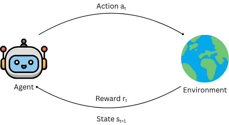
At each step $t$ the agent observes the current state $s_t \in \mathcal{S}$, takes action $a_t \in \mathcal{A}$, subsequently receives reward $r_t \in \mathbb{R}$ and is transitioned to the next state $s_{t+1}$ by the environment.

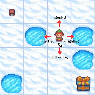
The agent's behavior is defined by a stochastic policy $\pi_\theta(a|s)$, which gives the probability of taking action $a$ in state $s$, parameterized by $\theta$.

From Rewards to Total Return

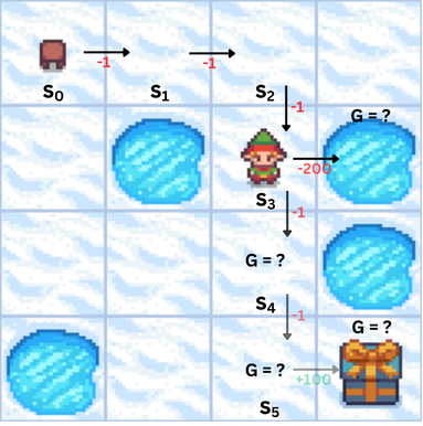
The agent’s objective is to maximize the total reward it receives over time, the return $G_t$. The return $G_t$ is the sum of rewards from time step $t$ onward:

$$G_t = r_t + r_{t+1} + r_{t+2} + \dots + r_T$$

But future rewards are often discounted. Why?

• Temporal Uncertainty: Future states and rewards are less certain (e.g., environment changes, agent timeout)
• Time Preference: Immediate rewards are often more valuable than delayed ones (e.g., economics, biology)
• Convergence Guarantees: Ensures the return (sum of rewards) remains finite in infinite-horizon problems
• Policy Stability: Encourages agents to prioritize near-term actions over distant, speculative ones

In essence, discounting helps to balance exploration and exploitation while making optimization tractable.

So, we use a discount factor $\gamma$ (where $0 \leq \gamma \leq 1$):

$$G_t = r_t + \gamma r_{t+1} + \gamma^2 r_{t+2} + \dots + \gamma^{T-t} r_T$$

From Total Return to Expected Return

The agent’s goal is to maximize the expected return (average total reward over many episodes):

$$J(\theta) = \mathbb{E}_{\tau \sim \pi_\theta} \left[ G_0 \right]$$

where $\tau$ represents a trajectory (sequence of states and actions), $\pi_\theta$ represents the policy (parameterized by $\theta$) and $G_0$ represents the total discounted reward from the start.

Deriving the Policy Gradient

The expected return $J(\theta)$ can be rewritten as

$$J(\theta) = \mathbb{E}_{\tau \sim \pi_\theta} \left[ G_0 \right] = \int_\tau P(\tau|\theta) G_0 d\tau$$

since $\pi_\theta$ represents a probability distribution, where $P(\tau|\theta)$ is the probability of trajectory $\tau$ under policy $\pi_\theta$.

Trajectory Probability

The probability of a trajectory $\tau$ is defined as

$$P(\tau|\theta) = P(s_0) \prod_{t=0}^T \pi_\theta(a_t|s_t) P(s_{t+1}|s_t, a_t)$$

where $P(s_0)$ is the initial state distribution and $P(s_{t+1}|s_t, a_t)$ is the environment dynamics (transition probability).

Gradient of the Objective

We want to find $\nabla_\theta J(\theta)$ w.r.t. $\theta$, which can be written as:

$$\nabla_\theta J(\theta) = \nabla_\theta \mathbb{E}_{\tau \sim \pi_\theta} \left[ G_0 \right] = \nabla_\theta \int_\tau P(\tau|\theta) G_0 \, d\tau$$

Since $G_0$ does not depend on $\theta$ (it is a function of the trajectory $\tau$, not the policy parameters), we can bring the gradient inside the integral.

$$\nabla_\theta J(\theta) = \int_\tau \nabla_\theta P(\tau|\theta) G_0 \, d\tau$$

The Log Derivative Trick

Recall that for any probability distribution $P(\tau|\theta)$, the following identity holds

$$\nabla_\theta P(\tau|\theta) = P(\tau|\theta) \nabla_\theta \log P(\tau|\theta)$$

This is due to the fact that $\frac{d}{dx} \left( \log x \right) = \frac{1}{x}$, with which we can similarly define $\nabla_\theta \log P(\tau|\theta)$

$$\nabla_\theta \log P(\tau|\theta) = \frac{\nabla_\theta P(\tau|\theta)}{P(\tau|\theta)} \implies \nabla_\theta P(\tau|\theta) = P(\tau|\theta) \nabla_\theta \log P(\tau|\theta)$$

This we can substitute back into the gradient of $J(\theta)$, yielding:

$$\nabla_\theta J(\theta) = \int_\tau P(\tau|\theta) \nabla_\theta \log P(\tau|\theta) G_0 \, d\tau$$

We realize this again is an expectation as $P(\tau|\theta)$ is again a probability distribution of trajectory $\tau$ under $\theta$, hence

$$\nabla_\theta J(\theta) = \mathbb{E}_{\tau \sim \pi_\theta} \left[ G_0 \nabla_\theta \log P(\tau|\theta) \right]$$

Computing $\nabla_\theta \log P(\tau|\theta)$

The only thing left now is to compute $\nabla_\theta \log P(\tau|\theta)$ given our earlier established form

$$P(\tau|\theta) = P(s_0) \prod_{t=0}^T \pi_\theta(a_t|s_t) P(s_{t+1}|s_t, a_t)$$

We take the log

$$\log P(\tau|\theta) = \log P(s_0) + \sum_{t=0}^T \left( \log \pi_\theta(a_t|s_t) + \log P(s_{t+1}|s_t, a_t) \right)$$

And then the gradient w.r.t. $\theta$

$$\nabla_\theta \log P(\tau|\theta) = \underbrace{\nabla_\theta \log P(s_0)}_{0} + \sum_{t=0}^T \left( \nabla_\theta \log \pi_\theta(a_t|s_t) + \underbrace{\nabla_\theta \log P(s_{t+1}|s_t, a_t)}_{0} \right)$$

As we realize that the initial state distribution $P(s_0)$ and the environment dynamics $P(s_{t+1}|s_t, a_t)$ do not depend on $\theta$, and in turn their gradients are 0, we can simplify to

$$\nabla_\theta \log P(\tau|\theta) = \sum_{t=0}^T \nabla_\theta \log \pi_\theta(a_t|s_t)$$

The Policy Gradient Theorem

Substituting back into the gradient of the objective:

$$\nabla_\theta J(\theta) = \mathbb{E}_{\tau \sim \pi_\theta} \left[ \left( \sum_{t=0}^T \nabla_\theta \log \pi_\theta(a_t|s_t) \right) G_0 \right]$$

But we can generalize this to any time step $t$ (since the return $G_t$ depends on future rewards):

$$\nabla_\theta J(\theta) = \mathbb{E}_{\tau \sim \pi_\theta} \left[ \sum_{t=0}^T \nabla_\theta \log \pi_\theta(a_t|s_t) G_t \right]$$

This is the Policy Gradient Theorem, which forms the basis of many RL algorithms and tells us how to compute the gradient of the expected return with respect to the policy parameters.

Monte Carlo Estimation of the Gradient

Since we can't compute the expectation exactly, we sample trajectories $\tau$ from the policy $\pi_\theta$ and approximate the gradient

$$\nabla_\theta J(\theta) \approx \frac{1}{N} \sum_{i=1}^N \sum_{t=0}^T \nabla_\theta \log \pi_\theta(a_{i,t}|s_{i,t}) G_{i,t}$$

where

• $N$ = number of sampled trajectories
• $a_{i,t}$ = action taken at time $t$ in trajectory $i$
• $G_{i,t}$ = return from time $t$ in trajectory $i$

The REINFORCE Algorithm

The REINFORCE algorithm uses this gradient estimate to update the policy:

1. Sample a trajectory $\tau = (s_0, a_0, r_0, s_1, a_1, r_1, \dots, s_T, a_T, r_T)$ using $\pi_\theta$.
2. Compute returns $G_t$ for each time step $t$.
3. Update the policy using gradient ascent:

$$\theta \leftarrow \theta + \alpha \sum_{t=0}^T \nabla_\theta \log \pi_\theta(a_t|s_t) G_t$$

where $\alpha$ is the learning rate.

Intuitively we can understand the derived formula such as

• $\nabla_\theta \log \pi_\theta(a_t|s_t)$ tells us how to change $\theta$ to increase the probability of action $a_t$ in state $s_t$.
• $G_t$ tells us how good the return was after taking action $a_t$.
• The product $\nabla_\theta \log \pi_\theta(a_t|s_t) G_t$ means:
  • If $G_t$ is positive (good outcome), we increase the probability of $a_t$ in $s_t$.
  • If $G_t$ is negative (bad outcome), we decrease the probability of $a_t$ in $s_t$.

Implementing REINFORCE

As we've become comfortable with the mathematical intricacies of Policy Gradients and the REINFORCE algorithm, we want to proceed with the implementation of it.

The Environment

Before implementing parts of the algorithm, we need to create a gymnasium environment we'd like to solve.

# Choose an environment
env_id = "CartPole-v1"
# env_id = "Acrobot-v1"
# env_id = "LunarLander-v3"

# Create the environment
env = gym.make(env_id, render_mode="rgb_array")

observation_space_dim = env.observation_space.shape[0]
action_space_dim = env.action_space.n

In addition, we need to make ourselves familiar with the observation and action space of the environment. These will be the dimensions our Policy Network is going to work with.

The Policy Network $\pi_\theta$

Next, we implement our policy network $\pi_\theta$, outputting the action probabilities for the given state.

class PolicyNetwork(nn.Module):
    def __init__(self, state_dim, action_dim, hidden_dim=16):
        super(PolicyNetwork, self).__init__()
        self.fc1 = nn.Linear(state_dim, hidden_dim)
        self.fc2 = nn.Linear(hidden_dim, action_dim)

    def forward(self, x):
        x = self.fc1(x)
        x = F.relu(x)
        x = self.fc2(x)
        x = F.softmax(x, dim=-1)
        return x

# Create a policy network instance
policy_net = PolicyNetwork(observation_space_dim, action_space_dim)

Taking an Action $a_t$

We defined the environment, we defined the policy network $\pi_\theta$. To take an action, we sample from our policy network $\pi_\theta$ given the current state $s_t$

def select_action(state, policy_net):
    state = torch.FloatTensor(state)
    probs = policy_net(state) # Get the action probabilites from policy
    dist = Categorical(probs) # Create categorical distribution over the actions
    action = dist.sample() # Sample an action from the categorical distribution
    log_prob = dist.log_prob(action) # Derive the log probability of the selected action

    return action.item(), log_prob

Our method yields both the action taken and the log probabilities of it for the gradient update later on.

Calculating the Returns $G_t$

For each action $a_t$ taken, we receive a reward $r_t$. These rewards are then used to calculate the total return $G_t$ of each step $t$, discounted by $\gamma$.

def compute_returns(rewards, gamma=0.99):
    returns = []
    R = 0
    
    # Process rewards in reverse order 
    for r in reversed(rewards):
        R = r + gamma * R # Discounted return at step t
        returns.insert(0, R) # Insert at beginning to maintain order

    returns = torch.FloatTensor(returns)
    
    # Normalize returns to reduce variance
    returns = (returns - returns.mean()) / (returns.std() + 1e-8)
    
    return returns

Sampling a Trajectory $\tau$

Now that we have all the distinct parts, we compose them to sample one full trajectory $\tau$ from the environment using our policy network $\pi_\theta$.

def sample_trajectory(env, policy_net):
    states, actions, rewards, log_probs = [], [], [], []
    state, _ = env.reset()

    done = False
    steps = 0
    
    # Run until episode ends or max steps are reached
    while not done and steps < env.spec.max_episode_steps:
        # Select an action based on the current state
        action, log_prob = select_action(state, policy_net)
        
        # Take the action in the environment
        next_state, reward, terminated, truncated, _ = env.step(action)

        # Store the trajectory
        states.append(state)
        actions.append(action)
        rewards.append(reward)
        log_probs.append(log_prob)

        # Update the state
        state = next_state

        done = terminated or truncated
        steps += 1

    return states, actions, rewards, log_probs

This method yields all the visited states, all the actions taken in each state, the rewards received and the log probabilities of each action.

Training the Agent

The only thing left to do is define how the agent is being trained. We iterate through a number of episodes, for each generating a distinct trajectory.

For each trajectory generated, we use the log probability of actions and multiply by the returns to get our gradient.

def train_reinforce(env, policy_net, num_episodes, gamma=0.99, lr=0.01):
    optimizer = torch.optim.Adam(policy_net.parameters(), lr=lr)

    for episode in range(num_episodes):
        # Sample a full trajectory
        states, actions, rewards, log_probs = sample_trajectory(env, policy_net)

        # Compute returns
        returns = compute_returns(rewards, gamma)

        # Compute policy loss
        policy_loss = []
        for log_prob, R in zip(log_probs, returns):
            # REINFORCE : -log_prob * return
            policy_loss.append(-log_prob * R)

        # Sum up the loss
        policy_loss = torch.stack(policy_loss).sum()

        # Update policy
        optimizer.zero_grad()
        policy_loss.backward()
        optimizer.step()

        # Print progress
        if episode % 10 == 0:
            print(f"Episode {episode}, Total Reward: {sum(rewards):.2f} {'Solved' if sum(rewards) >= env.spec.reward_threshold else ''}")

    return policy_net

The gradient is then backpropagated through our policy network $\pi_\theta$ to improve the policy wrt. the experience gathered by the trajectory.

Evaluating the Agent

After we've successfully trained our agent, we most likely want to see how it performs. For our gymnasium environment selection we can even generate a video of our agents performance.

def evaluate(env, policy_net):
    # Wrap environment to record a video
    env = RecordVideo(env, video_folder=f"videos", name_prefix=f"{env.spec.id}")
    
    state, _ = env.reset()
    total_reward = 0

    done = False
    # Run until the episode ends
    while not done:
        # Select an action based on our policy
        with torch.no_grad(): # Do not track gradients in evaluation
            action, _ = select_action(state, policy_net)
        
        # Take action in environment
        next_state, reward, terminated, truncated, _ = env.step(action)
        total_reward += reward
        state = next_state
        
        done = terminated or truncated

    print(f"Total Reward: {total_reward:.2f}")

    env.close()

We use torch.no_grad() to disable gradient tracking during evaluation.

Seeing the Result

If all goes well, we can marvel at the performance of our trained agent(s).

CartPole-v1

Acrobot-v1

LunarLander-v3

Next Steps

This implementation provides a solid foundation for understanding Policy Gradient methods in deep reinforcement learning. 

While REINFORCE is a simple and effective algorithm, there are of course several ways to improve both the implementation and the algorithm itself.

• We might want to add a baseline (like a value function) to reduce variance in the gradient estimates.
• We might move one step further and extend this approach to an Actor-Critic model which combines policy gradients with value function learning.
• We could implement different exploration strategies such as $\epsilon$-greedy exploration or add entropy-regularization for better state space exploration
• We should furher, explore more advanced algorithms such as Proximal Policy Optimization (PPO), SAC (Soft Actor-Critic), DQN (Deep Q-Networks), and many more.

The full source code is available on Gitlab as an interactive Jupyter Notebook.