Introduction to Content-Based Recommender Systems

Content-Based Recommender Systems are a fundamental class of recommendation engines that can generate personalized suggestions by analysing intrinsic features of items preferred by users.

Unlike collaborative filtering, which relies on user-item interaction data from multiple users, content-based filtering focuses solely on the attributes of items and individual user profiles. This makes it especially valuable in scenarios where user interaction data is sparse or unavailable, such as cold-start problems for new users or items.

Content-Based Filtering operates by finding similar items matching those users have looked or liked in the past, but matching them solely on content-based features such as text description or other metadata information.

The independence of other users data in contrast to collaborative filtering, makes content-based filtering especialy robust against data sparsity and privacy concerns, making it widely applicable in fields such as personalized news feeds, e-commerce product recommendations and document retrieval systems.

Handling Documents: Tokens, N-grams and Index Terms

At the core of content-based filtering lies the representation of documents in a form that enables efficient retrieval and comparison.

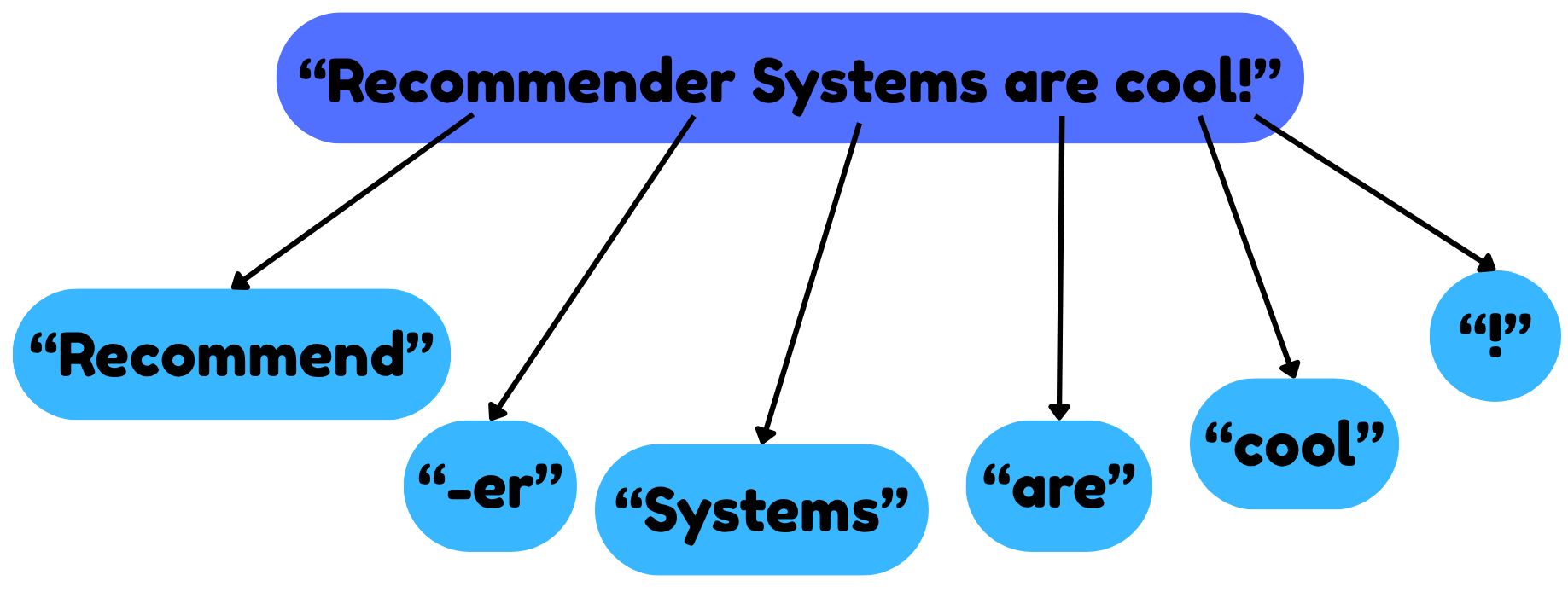
This begins with tokenization, the process of breaking down text into smaller semantic units. Tokens can be words, phrases or even sub-words, depending on the application.

Tokenization is essential for transforming unstructured text into a format suitable for computational processing, indexing, and similarity measurement.

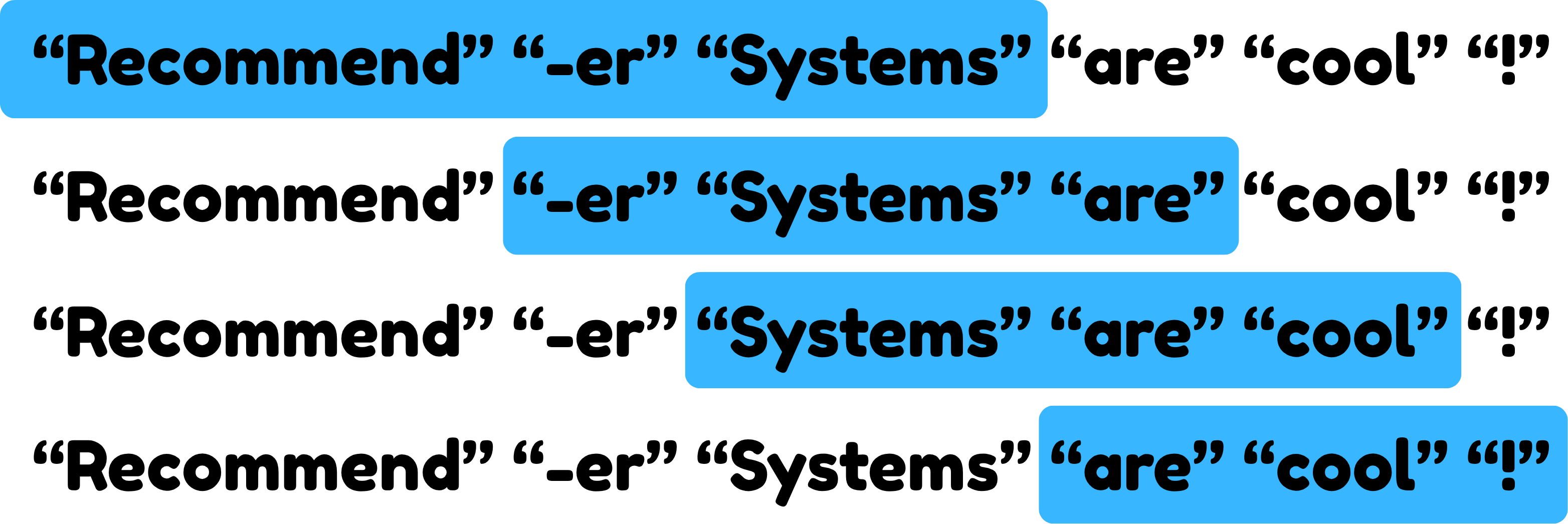
N-grams extend this concept by considering contiguous sequences of $n$ tokens, capturing local context and word relationships. For instance, bigrams (2-grams) and trigrams (3-grams) help in predictive text applications and improve the accuracy of document matching by encoding word co-occurence patterns. N-grams are pivotal in information retrieval tasks, where they assist in ranking documents based on the relevance of n-gram patterns to user queries.

Index terms are the vocabulary of terms derived from tokenization and normalization processes, used to represent documents in an information retrieval system. These terms are often normalized (e.g. case folding, stemming) to reduce redundancy and improve matching accuracy. Index terms enable the system to efficiently assess the relevance of documents to queries by focusing on the most meaningful and discriminative terms.

In our example these might be "recommend", "system" and "cool" which could be used to refer to the original document "Recommender Systems are cool!".

Text Preprocessing: Stopword Removal, Case Folding and Stemming

Text preprocessing is a critical step in content-based filtering, which aims to enhance the quality of document representation and recommendation accuracy.

Three of the most widely used pre-processing methods are:

• Stopword Removal: Eliminating common words (e.g. "the", "and", "a") which carry little semantic meaning to reduce noise and enhance the focus on meaningful content. This also reduces vocabulary size.
• Case Folding: Converting all text to lowercase standardizes the input, preventing redundant terms due to case differences (e.g. "Cat" vs "cat"). This, however, might be misleading in some cases. ("Apple" vs "apple")
• Stemming: Reducing words to their root form (e.g. "run" for "running") consolidates variants of the same word, improving the accuracy of classifiers and additionally reducing vocabulary size.

These techniques, among others, collectively enhance the performance of content-based recommender systems by reducing noise, improving term matching and lowering computational complexity.

The Bag of Words Model: Representing Text Data

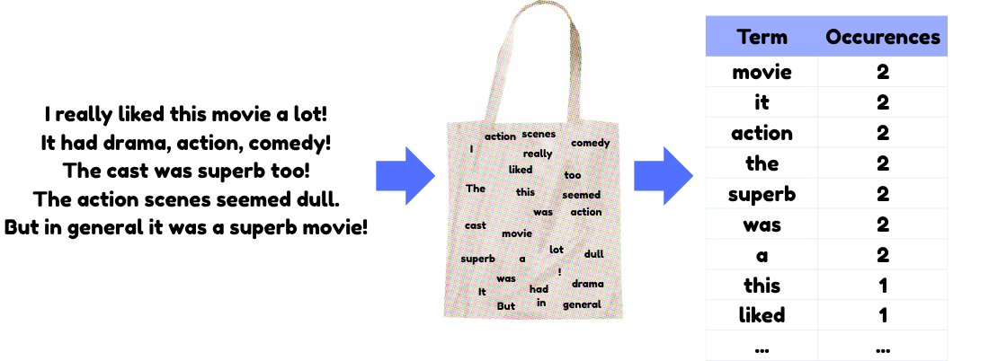
The Bag of Words (BoW) model is a widely used method to represent text documents as numerical vectors. It treats a document as an unordered collection of words, where the frequency of each word in the document is counted, and word order and context are disregarded.

It converts text into a vector space where each dimension corresponds to a unique word in the vocabulary, and the value represents the word's frequency in the document.

BoW is favoured for its simplicity and interpretability, making it a well suited for document classification, sentiment analysis and spam detection. However, it suffers from several limitations:

• Loss of word order and context: By ignoring word order and syntax, BoW loses the semantic relationships between words, which can reduce the accuracy of document representation.
• Curse of dimensionality: As the vocabulary size grows, BoW vectors become high-dimensional and sparse, leading to computational inefficiencies and reduced accuracy.
• Equal weighting: BoW treats all words equally, which can overemphasize frequent but less meaningful words.

Despite these limitations, BoW remains a foundational technique for converting text into numerical features suitable for machine learning algorithms.

Document Modelling Using the Vector Space Model

The Vector Space Model (VSM) represents documents and queries as vectors in a high-dimensional space, where each dimension corresponds to a unique term in the vocabulary, as in BoW.

Contrary to BoW, VSM serves as a generalization. VSM can be applied similarly to BoW is by counting word occurences, but generally is used with term-weighting methods like TF-IDF.

Hence, the value in each dimension reflects the frequency or weight of the term in the document or query. The comparison of documents and queries is based on vector similarity measures, such as cosine similarity.

Think of the following set of documents:

• Document 1: "The cat sat on the mat."
• Document 2: "The dog played with the ball."
• Document 3: "The cat chased the dog."

First we create a vocabulary of all unique terms in the documents.

$$\{\text{"the"}, \text{"cat"}, \text{"sat"}, \text{"on"}, \text{"mat"}, \text{"dog"}, \text{"played"}, \text{"with"}, \text{"ball"}, \text{"chased"} \}$$

Each document is represented as a vector in this 10-dimensional space, with each dimension corresponding to a term in the vocabulary. The value in each dimension can be a simple count of how often the term appears in the document, or derived by other term weighting techniques.

• Document 1 Vector: $\begin{bmatrix}2 & 1 & 1 & 1 & 1 & 0 & 0 & 0 & 0 & 0\end{bmatrix}$
  • "The" appears 2 times, "cat" appears 1 time, ...
• Document 2 Vector: $\begin{bmatrix} 2 & 0 & 0 & 0 & 0 & 1 & 1& 1 & 1 & 0\end{bmatrix}$
  • "The" appears 2 times, "dog" appears 1 time, "cat" doesn't appear at all, ...
• Document 3 Vector: $\begin{bmatrix} 2 & 1 & 0 & 0 & 0 & 1 & 0 & 0 & 0 & 1\end{bmatrix}$
  • "The" appears 2 times, "dog" and "cat" appear 1 time each, ...

Now we can accept queries such as "cat and dog" and map it to a query vector:

• Query Vector: $\begin{bmatrix} 0 & 1 & 0 & 0 & 0 & 1 & 0 & 0 & 0 & 0\end{bmatrix}$
  • "cat" appears 1 time, "dog" appears 1 time, "and" is not in our vocabulary

Based on this query vector we can perform similarity calculations to our document vectors and retrieve the best matching documents.

VSM is fundamental in information retrieval, document classification and word embeddings. It allows for efficient document categorization and relevance ranking by capturing semantic meaning of words through their co-occurence patterns.

However, it's important to note that VSM, similarly to BoW, greatly suffers from the curse of dimensionality for big vocabularies and assumes term independence, which can limit its accuracy in capturing complex semantic relationship.

Term Weighting and Monotonicity Assumptions

Term weighting assigns importance to terms based on their frequency and distribution across documents.

The most prominent weighting scheme is TF-IDF (Term Frequency - Inverse Document Frequency), which balances the frequency of a term in a document (TF) with its rarity across the entire corpus (IDF). This weighting scheme helps in emphasizing terms that are frequent in the document but rare overall, improving accuracy of document retrieval and recommendation.

When discussing term weighting schemes like TF-IDF, certain monotonicity assumptions are often considered to understand how term importance is calculated and interpreted.

• IDF Assumption: Less common words are just as influential as common ones. A word is more important to a document if it appears in fewer documents overall.
• TF Assumption: Repeated words in a document are just as important as words that appear only once. The more a word appears in a document, the more important it is to that document.
• Normalization Assumption: The length of a document doesn't make it more important. We shall adjust for document length when comparing how similar two documents are, or a document and a search query.

Term Frequency - Inverse Document Frequency (TF-IDF)

Term Frequency (TF) measures how often a term appears in a document normalized by the document length.

$$\text{TF(t, d)} = \frac{\text{Number of times term t appears in document d}}{\text{Total number of terms in document d}}$$

TF captures the importance of a term within a document but does not account for its commonness accross documents.

Inverse Document Frequency (IDF) measures the rarity of a term across the corpus.

$$\text{IDF(t, D)} = \log \left( \frac{\text{Total number of documents in corpus D}}{\text{Number of documents containing term t}} \right)$$

IDF reduces the weight of common words and increases the weight of rare words, improving the discriminative power of terms.

Term Frequency - Inverse Document Frequency (TF-IDF) combines TF and IDF to assign a weight to each term.

$$\text{TF-IDF(t, d, D)} = \text{TF(t, d)} \times \text{IDF(t, D)}$$

TF-IDF is widely used in information retrieval and recommender systems to improve the relevance of recommendations by emphasizing meaningful terms.

Zipf's Law and Its Relevance to Term Distribution

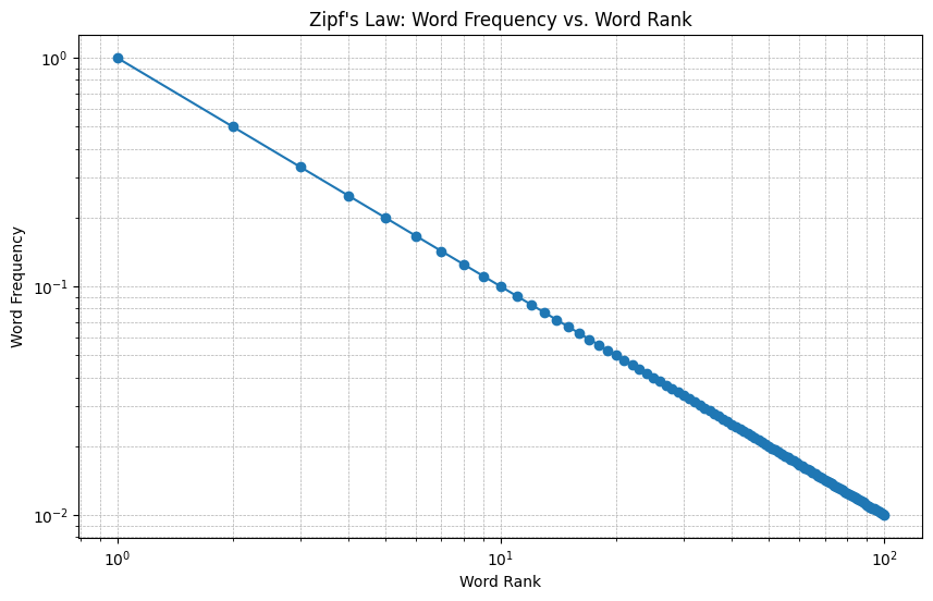
Zipf's law states that when a list of measured values is sorted in decreasing order, the value of the $n$-th entry is approximately inversely proportional to $n$.

$$\mathsf{word\ frequency} \propto \frac {1}{\mathsf {word\ rank}}$$

• Zipf's law aids in improving search algorithm efficiency by focusing on high-frequency terms.
• … text compression by prioritizing frequent words
• … search engine optimization by targeting high-ranking keywords
• … language modelling and text classification by focusing on the most meaningful terms.

In summary, Zipf's law helps in identifying the most important elements in a dataset, allowing for more efficient data processing, storage and analysis.

Similarity Measurement Techniques

Similarity measures help quantify how closely related documents or items are, which is essential for content-based filtering and recommendation.

There exist multiple similarity measurement techniques of which the most common ones are:

• Cosine Similarity: Measures the cosine of the angle between two vectors, ranging from -1 to 1. Used in document classification, sentiment analysis, and recommender systems to measure vector orientation similarity.

$$\text{cosine similarity}(\mathbf{A}, \mathbf{B}) = \frac{\mathbf{A} \cdot \mathbf{B}}{\|\mathbf{A}\| \|\mathbf{B}\|} = \frac{\sum_{i=1}^{n} A_i B_i}{\sqrt{\sum_{i=1}^{n} A_i^2} \sqrt{\sum_{i=1}^{n} B_i^2}}$$

• Jaccard Similarity (Intersection over Union): Measures the overlap between two sets. Useful for binary data and clustering tasks.

$$J(A, B) = \frac{|A \cap B|}{|A \cup B|}$$

• Euclidean Distance: Measures the straight-line distance between two vectors. Applied in clustering, classification, and customer segmentation.

$$d(\mathbf{p}, \mathbf{q}) = \sqrt{\sum_{i=1}^{n} (q_i - p_i)^2}$$

Advanced Topic Modelling Techniques

Representing and comparing textual content, in pure form, involves dealing with sparse high-dimensional and sometimes noisy data, which can hinder yielding good results for complex use cases or those requiring particularly robust solutions.

Advanced topic modelling techniques such as Latent Semantic Analysis (LSA), Probabilistic Latent Semantic Analysis (pLSA) and Latent Dirichlet Allocation (LDA) have emerged as powerful tools to address these challenges.

These methods aim to uncover latent semantic structures within text corpora, enabling more accurate recommendation results.

Latent Semantic Analysis (LSA)

Latent Semantic Analysis (LSA) is a dimensionality reduction technique rooted in linear algebra which identifies latent semantic relationships between words and documents. It operates on the distributional hypothesis: words with similar meanings tend to appear in similar contexts.

LSA constructs a term-document matrix $\mathbf{X}$, in which rows correspond to unique words and columns to the documents of the corpus, typically weighted by term frequency-inverse document frequency (tf-idf) to emphasize important terms.

LSA decomposes the term-document matrix $\mathbf{X}$ using Singular Value Decomposition (SVD)

$$\mathbf{X} = \mathbf{U} \mathbf{\Sigma} \mathbf{V^T}$$

where $\mathbf{U}$ and $\mathbf{V}$ are orthogonal matrices, and $\mathbf{\Sigma}$ is a diagonal matrix of singular values.

The rank reduction step selects the top $k$ singular values and corresponding vectors, yielding a low-rank approximation

$$\mathbf{X_k} = \mathbf{U_k}\mathbf{\Sigma_k}\mathbf{V_k^T} $$

This approximation captures the most significant latent semantic dimensions, enabling efficient comparison of documents and terms in a reduced space.

LSA is widely used in information retrieval, document clustering, and text summarization. In content-based filtering, LSA helps measure semantic similarity between items (e.g., movie plots) and user queries or profiles, improving recommendation accuracy beyond simple word matching.

Probabilistic Latent Semantic Analysis (pLSA)

Probabilistic Latent Semantic Analysis (pLSA) extends LSA by modeling the joint probability of words and documents as a mixture of latent topics. Each topic is a multinomial distribution over words, and documents are modeled as mixtures of these topics.

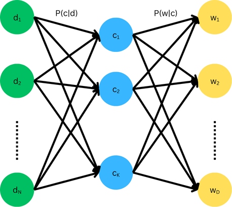
In pLSA the joint probability $P(w,d)$ can be expressed by summing over all possible latent topics $c$.

$$P(w,d) = \sum_c P(w,d,c)$$

This can be further factorized to

$$P(w,d) = \sum_c P(d) P(c | d) P (w | c, d)$$

Applying the conditional independence assumption of pLSA, which states that the words $w$ are independent of document $d$ given topic $c$, which means $P(w| c, d) = P (w | c)$, we can further simplify.

$$\begin{align*} P(w,d) &= \sum_c P(d) P(c | d) P(w | c) \\&= P(d) \sum_c P(c | d) P(w | c)\end{align*}$$

Which represents the core model of pLSA, yielding the following model parameters:

• $P(d)$: The prior probability of selecting document $d$. Usually estimated from data, not learned.
• $P(c |d)$: The probability of topic $c$ in document $d$. Learned from data. Tells us what topics are present in each document.
• $P(w|c)$: The probability of word $w$ given topic $c$. Learned from data. Tells us how each topic "speaks".

pLSA learns the model parameters using Expectation-Maximinzation (EM), which iteratively refines topic assignments and word-topic probabilities.

Crucially, $P(c)$, the marginal probability of topic $c$ is not modeled explicitly in pLSA, which is a key difference from models like Latent Dirichlet Allocation (LDA), which puts priors over topics.

Latent Dirichlet Allocation (LDA)

Latent Dirichlet Allocation (LDA) is a generative statistical model which assumes each document in a corpus is a mixture of a small number of topics, and each topic is characterized by a distribution over words, as in pLSA. LDA however, introduces Dirichlet priors on topic distributions.

To better understand LDA, it's helpful to use plate notation, a graphical representation often used to describe probabilistic graphical models.

• Outer Plate: Represents the documents in the corpus
• Inner Plate: Represents the repeated word positions within each document.

In the plate notation, words $W$ are grayed out to indicate the fact that these are the only observable variables, while the other variables are latent (hidden).

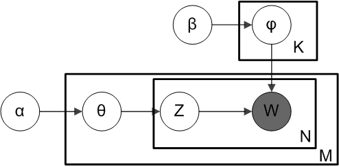
The variables of the model are defined as follows:

• $M$: Number of documents
• $N$: Number of words in a given document
• $K$: Number of expected topics
• $\alpha$: Parameter of the Dirichlet prior on the per-document topic distributions. (Prior weight of topics in a document)
• $\beta$: Parameter of the Dirichlet prior on the per-topic word distribution. (Prior weight of words in a topic)
• $\theta_i$: Topic distribution for document $i$.
• $\psi_k$: Word distribution for topic $k$.
• $z_{ij}$: Topic for the j-th word in document $i$
• $w_{ij}$: Specific word

Following the given model the total probability is defined as

$$P(W, Z, \theta, \psi, \alpha, \beta) = \prod_{i=1}^K P(\psi_i; \beta) \prod_{j=1}^M P(\theta_j; \alpha) \prod_{t=1}^N P(Z_{j,t} | \theta_j) P(W_{j,t} | \theta_{Z_{j,t}})$$

Latent Dirichlet Allocation is most commonly, as pLSA, trained via Expectation Maximization (EM) or alternatively via Gibbs Sampling (Markov chain Monte Carlo algorithm).

The Generative Process

To infer the topics in a corpus, LDA imagines a generative process whereby documents are created:

• Choose Topic Distributions: For each document, choose a topic distribution $\theta_i$ from a Dirichlet distribution parameterized by $\alpha$
• Choose Word Distributions: For each topic, choose a word distribution $\psi_k$ from a Dirichlet distribution parameterized by $\beta$.
• Generate Words: For each word position in each document:
  • Choose a topic $z_{ij}$ from a multinomial distribution parameterized by $\theta_i$.
  • Choose a word $w_{ij}$ from a multinomial distribution parameterized by $\psi_k$, where $k$ is the topic chosen in the previous setup.

This process results in a corpus of documents, each with a mixture of topics, and each topic with a mixture of words.

Dirichlet Prior

The use of Dirichlet priors serves several important purposes:

• Sparsity and Smoothness: Dirichlet priors encourage sparsity in the topic-word and document-topic distributions. This means that only a few topics are likely to be dominant in a document, and only a few words are likely to be dominant in a topic. This sparsity makes the model more interpretable and often more realistic, as documents typically focus on a few main themes.
• Regularization: Dirichlet priors act as a form of regularization. They prevent the model from overfitting to training data by discouraging extreme values in the distributions.
• Handling of Rare Words: Without a distribution such as the Dirichlet distribution, rare words might be ignored or treated as noise. The priors ensure that even rare words have a non-zero probability of being associated with a topic.

The increase in topic quality due to the assumed Dirichlet distribution of topics is clearly measurable.

Conclusion

In conclusion, Content-Based Recommender Systems personalize recommendations using various item features and user preferences, ideal for scenarios with limited user data.

Techniques like tokenization, VSM and Bag of Words allow to structure textual data, while preprocessing helps reducing vocabulary size and ambiguity.

Term weighting, especially TF-IDF improve relevance by emphasizing key terms of documents.

Similarity measures and topic modeling techniques like LSA and LDA refine recommendations further.