Collaborative Filtering in Recommender Systems

In today's age, recommender systems are integral to enhancing user experience by suggesting products, services or content tailored to individual preferences. These systems are widely used across various domains such as e-commerce, streaming services, and social media platforms. One of the most effective and widely adopted techniques in recommender systems is Collaborative Filtering (CF).

In this post, we aim to provide an in-depth understanding of collaborative filtering, including different types and it's significance in the realm of recommender systems.

Introduction to Recommender Systems

Recommender systems are designed to predict user prefernces and provide personalized recommendations. They leverage data on user behaviour, preferences, and interactions to suggest items that users are likely to find appealing. Broadly speaking, there are several types of recommender systems, including:

• Collaborative Filtering: This technique aims to make automatic predictions (filtering) about the interests of a users by collecting preferences from many users (collaborative). The underlying assumption is that users who agreed strongly on items in the past likely find similar kinds of items interesting.
• Content-Based Filtering: This approach recommends items similar to those a user has liked in the past, based on the features or content of the items. Users who might frequently watch action movies, might find movies of similar content type (Action genre with high similarity on the movie description) interesting.
• Context-Aware Recommender Systems: These systems take into account the context in which recommendations are made, providing more relevant and personalized suggestions. Context can include various factors such as time, location, device, social setting, or even the users emotional state.
• Hybrid Recommender Systems: These systems combine the above mentioned systems to improve accuracy and performance of their recommendations. By leveraging the strengths of each method, hybrid systems can provide more robust and personalized recommendations.

Collaborative Filtering: An Overview

Collaborative filtering is one of the most widely used approaches for building recommender systems. It is applicable to many domains and does not require explicit domain knowledge.

CF collects user feedback in the form of explicit or implicit ratings of items and uses these ratings collectively to determine whether to recommend an item to a user or not.

Collaborative filteing can broadly be categorized into memory-based and model-based collaborative filtering.

Memory-Based Collaborative Filtering

Memory-based collaborative filtering, also known as neighborhood-based collaborative filtering, relies on user-item interactions stored in memory to make predictions, hence no "model" is built but predictions are made on the fly based on the stored rating data in a nearest neighbor approach.

It can be further divided into user-based and item-based approaches.

User-Based Collaborative Filtering

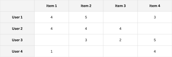
In user-based collaborative filtering, the goal is to predict the rating $r_{u,i}$ that a user $u$ would give to item $i$ based on the ratings given by similar users.

Typically the similarity between users is calculated using metrics such as the Pearson correlation coefficient.

The Pearson correlation coefficient between two users $u$ and $v$ is given by:

$$ \text{sim}(u, v) = \frac{\sum_{i \in I_{u,v}} (r_{u,i} - \bar r_{u})(r_{v,i} - \bar r_v)}{\sqrt{\sum_{i \in I_{u,v}} (r_{u,i} - \bar r_u)^2} \sqrt{\sum_{i \in I_{u,v}} (r_{v,i} - \bar r_v) ^2}}$$

where $I_{u,v}$ is the set of items rated by both users $u$ and $v$, $r_{u,i}$ defines the rating given by user $u$ to item $i$, and $\bar r_u$ is the average rating given by user $u$. The metrics ranges from -1 to +1 indicating similarity or dissimilarity strength, and already accounts for individual users rating bias (users that might generally tend to give lower/higher ratings or stay more neutral in their ratings).

Once the similarities between users are calculated, the predicted rating $\hat r_{u,i}$ for user $u$ and item $i$ can be computed as a weighted sum of the ratings given the the most similar users like:

$$\hat r_{u,i} = \bar r_u + \frac{\sum_{v \in N(u)} \text{sim(u,v)} (r_{v,i} - \bar r_v)}{\sum_{v \in N(u)} \text{sim(u,v)}}$$

where $N(u)$ is the set of the $k$ most similar users to user $u$.

It starts with $\bar{r}_u$​, the user's average rating, and adjusts it based on deviations from similar users' ratings. The similarity measure, $\text{sim}(u,v)$, ensures that more similar users have a greater impact. The term $r_{v,i} - \bar{r}_v$ accounts for individual rating biases, while $N(u)$ focuses on the most similar users. The weighted sum of these deviations, normalized by the sum of similarities, provides a balanced and personalized prediction.

Item-Based Collaborative Filtering

In item-based collaborative filtering, the goal is to predict the rating $r_{u,i}$ that user $u$ would give to item $i$ based on the ratings given to similar items. The similarity between items is typically calculated using cosine similarity or adjusted cosine similarity, which does account for different item popularities as well as user rating biases.

The adjusted cosine similarity between two items $i$ and $j$ is given by:

$$ \text{sim(i,j)} = \frac{\sum_{u \in U_{i,j}} (r_{u,i} - \bar r_u) (r_{u,j} - \bar r_u)}{\sqrt{\sum_{u \in U_{i,j}} (r_{u,i} - \bar r_u)^2} \sqrt {\sum_{u \in U_{i,j}} (r_{u,j} - \bar r_u)^2}}$$

where $U_{i,j}$ is the set of users who have rated both items $i$ and $j$.

Once the similarities between items are calculated, the predicted rating $\hat r_{u,i}$ for user $u$ and item $i$ can be computed as a weighted sum of the ratings given to the most similar items like:

$$\hat r_{u,i} = \frac{\sum_{j \in N(i)} \text{sim(i,j)} r_{u,j}}{\sum_{j \in N(i)} \text{sim(i,j)}}$$

where $N(i)$ is the set of the $k$ most similar items to item $i$.

In summary, memory-based collaborative filtering methods store all ratings and calculate new rating predictions on the fly using nearest neighbor approach. On the upside, these systems are very interpretable as a single rating prediction can be traced back exactly to it's origins, however we must also acknowledge that this approach gets very memory-demanding quickly.

Other problems are also data sparsity (sparse rating data yields high uncertainty on the real neighborhood and similarity of users and items), "cold-start" problem (new users have no similarty, as they haven't rated anything yet), curse of dimensionality, ...

Model-Based Collaborative Filtering

Model-based collaborative filtering involves building a model from the user-item interactions data to make predictions. This approach can handle some of the limitations such as data sparsity and scalability of memory-based methods.

Latent Factor Models

Latent factor models try to explain ratings by putting both users and items in an $d$-dimensional restricted space of factors derived from the ratings patterns seen in the user-item data matrix.

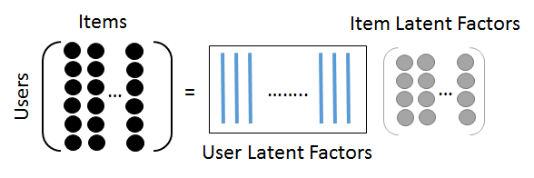
This projection into latent space allows for grouping rating patterns and derive user and item characteristcs such as age or gender, but also genre, purpose or category depending on the item type.

Matrix Factorization

Matrix factorization is a popular technique for model-based collaborative filtering. It factorizes the user-item matrix $R$ into two lower-dimensional matrices $P$ and $Q$ representing user and item latent factors, respectively.

The user-item rating matrix $R$ can be approximated as:

$$R = P^T Q$$

where $P$ is a $d \times m$ matrix representing the user latent factors, $Q$ is a $d \times n$ matrix representing the item latent factors. $m$ describes number of users, $n$ is the number of items, and $d$ is the dimensionality of the latent space.

After we got $P$ and $Q$, predictions can be made for all users $u$ and items $i$ via $\hat r_{u,i} = p_u^T q_i $.

The goal of matrix factorization is to minimize the following loss function:

$$\mathcal{L} = \sum_{(u,i) \in K} (r_{u,i} - \hat{r}_{u,i})^2 + \lambda \left( \sum_{u} \|p_u\|^2 + \sum_{i} \|q_i\|^2 \right)$$

where $K$ is the set of observed ratings, $r_{u,i} \in R$ is the observed rating, $\hat r_{u,i} = p_u^T q_i$ is the predicted rating utilizing the latent factors.

$p_u$ is the latent factor vector for user $u$ whereas $q_i$ is the latent factor vector for item $i$.

The regularization term denoted by $ \sum_{u} \|p_u\|^2 + \sum_{i} \|q_i\|^2 $ is to prevent overfitting by penalizing the magnitudes of the latent factor vectors, it adds a cost associated with the Euclidean norms (or lengths) of these vectors, encouraging the model to keep the values of $p_u$ ​and $q_i$ ​small.

The regularization parameter $\lambda$ controls the strength of this penalty, helping to balance the fit of the model to the observed data and the simplicity of the latent factors.

Singular Value Decomposition (SVD)

Singular Value Decomposition (SVD) is a specific type of matrix factorization that decomposes a given matrix, $R$ in our case, into three matrices such as:

$$R = U \Sigma V^T$$

where $U$ is a $m \times m$ orthogonal matrix representing the user latent factors, $\Sigma$ is a $m \times n$ diagonal matrix containing the singular values, and $V$ is a $n \times n$ orthogonal matrix representing the item latent factors.

The predicted rating $\hat r_{u,i}$ can then be computed like:

$$\hat r_{u,i} = \sum_{k=1}^d u_{u,k} \sigma_k v_{i,k}$$

where $u_{u,k}$ is the $k$-th component of the user latent factor vector for user $u$, $\sigma_k$ is the $k$-th singular value and $v_{i,k}$ is the $k$-th component of the item latent factor vector for item $i$.

While Singular Value Decomposition is a powerful mathematical tool for matrix decomposition, it has serveral limitations when applied to real-world recommender systems such as data-sparsity (user-item matrix will likely always be sparse), scalability issues (user-item matrix grows quickly, computational efforts increase), inherent lack of regularization and difficulties with dynamic data.

Gradient Descent

Thus we might want to directly estimate the latent user vectors $P$ and latent item vectors $Q$ only from known ratings $r_{u,i} \in R$ by directly minimizing the matrix factorization loss objective defined above.

The updates needed for the user and item latent factor vectors using gradient descent can be defined as:

$$p_u \leftarrow p_u - \eta \frac{\partial \mathcal{L}}{\partial p_u}$$

$$q_i \leftarrow q_i - \eta \frac{\partial \mathcal{L}}{\partial q_i}$$

where $\eta$ is the learning rate, and the gradients are computed as:

$$\frac{\partial \mathcal{L}}{\partial p_u} = -2 \sum_{i \in I_u} (r_{u,i} - \hat{r}_{u,i}) q_i + 2 \lambda p_u$$

$$\frac{\partial \mathcal{L}}{\partial q_i} = -2 \sum_{u \in U_i} (r_{u,i} - \hat{r}_{u,i}) p_u + 2 \lambda q_i$$

where $I_u$ is the set of items rated by user $u$, and $U_i$ is the set of users who have rated item $i$.

Incorporating User and Item Biases

As done for the methods and algorithms before, we have to take user and item biases into consideration when estimating rating $\hat r_{u,i}$.

In order to do so, we introduce $\mu$ acting as global average rating, $b_i$ accounting for item bias and $b_u$ accounting for user bias. Hence the new loss objective becomes:

$$\mathcal{L} = \sum_{(u,i) \in K} (r_{u,i} - \hat r_{u,i} - \mu - b_u - b_i)^2 + \lambda \left( \sum_u \|p_u\|^2 + \sum_i \|q_i\|^2 + \sum_u b_u^2 + \sum_i b_i^2 \right)$$

The updates for the user and item latent factor vectors, as well as the biases, using gradient descent are given by:

$$p_u \leftarrow p_u - \eta \frac{\partial \mathcal{L}}{\partial p_u}$$

$$q_i \leftarrow q_i - \eta \frac{\partial \mathcal{L}}{\partial q_i}$$

$$b_u \leftarrow b_u - \eta \frac{\partial \mathcal{L}}{\partial b_u}$$

$$b_i \leftarrow b_i - \eta \frac{\partial \mathcal{L}}{\partial b_i}$$

where the gradients are computed as:

$$\frac{\partial \mathcal{L}}{\partial p_u} = -2 \sum_{i \in I_u} (r_{u,i} - \hat r_{u,i} - \mu - b_u - b_i) q_i + 2 \lambda p_u$$

$$\frac{\partial \mathcal{L}}{\partial q_i} = -2 \sum_{u \in U_i} (r_{u,i} - \hat r_{u,i} - \mu - b_u - b_i) p_u + 2 \lambda q_i$$

$$\frac{\partial \mathcal{L}}{\partial b_u} = -2 \sum_{i \in I_u} (r_{u,i} - \hat r_{u,i} - \mu - b_u - b_i) + 2 \lambda b_u$$

$$\frac{\partial \mathcal{L}}{\partial b_i} = -2 \sum_{u \in U_i} (r_{u,i} - \hat r_{u,i} - \mu - b_u - b_i) + 2 \lambda b_i$$

By incorporating biases and regularization into the gradient descent framework, the model can learn more accurate and interpretable latent factors, leading to better recommendations.

In summary, model-based collaborative filtering approaches are particularly effective for handling large datasets, providing real-time recommendations by leveraging pre-computed rating models, making them suitable for dynamic environments. However, as user ratings and item characteristics change over time, strategies for updating the model are crucial.

Summary

Collaborative filtering-based recommender systems are well-established and extensively researched. They offer several advantages:

• Domain-independent, making them versatile across different fields
• No need for knowledge engineering, simplifying implementation

However, there are also notable challenges:

• Require a user base or community to function effectively
• Depend heavily on rating data, where sparsity can be a significant issue
• "Cold-start" problems make it struggle with new users or items that lack sufficient interaction data.