The Transformer Architecture

The Transformer architecture, introduced by the seminal paper "Attention is All You Need" by Vaswani et al. (2017), revolutionized natural language processing (NLP) and deep learning.

Attention Is All You Need

The dominant sequence transduction models are based on complex recurrent or convolutional neural networks in an encoder-decoder configuration. The best performing models also connect the encoder and decoder through an attention mechanism. We propose a new simple network architecture, the Transformer, based solely on attention mechanisms, dispensing with recurrence and convolutions entirely. Experiments on two machine translation tasks show these models to be superior in quality while being more parallelizable and requiring significantly less time to train. Our model achieves 28.4 BLEU on the WMT 2014 English-to-German translation task, improving over the existing best results, including ensembles by over 2 BLEU. On the WMT 2014 English-to-French translation task, our model establishes a new single-model state-of-the-art BLEU score of 41.8 after training for 3.5 days on eight GPUs, a small fraction of the training costs of the best models from the literature. We show that the Transformer generalizes well to other tasks by applying it successfully to English constituency parsing both with large and limited training data.

arXiv.orgAshish Vaswani

Unlike traditional recurrent neural networks (RNNs) and Convolutional Neural Networks (CNNs), Transformers rely entirely on self-attention mechanisms to process sequential data, enabling parallelization and superior performance in tasks like machine translation, text generation, and more.

In this blog post, we want to dive deep into the Query-Key-Value relationships that power the self-attention mechanism of transformers, explain the structure of the transformer layers and its components, and discuss the different variants of encoder and decoder transformers.

$\mathbf{Q}$ueries , $\mathbf{K}$eys, and $\mathbf{V}$alues

At the heart of the Transformer lies the attention mechanism, which allows the model to dynamically weigh the importance of different input tokens when producing an output. Unlike fixed-weight operations (e.g., convolutions), attention is data-dependent, enabling the model to focus on relevant parts of the input sequence.

Scaled Dot-Product Attention

The most fundamental form of attention in Transformers is the scaled dot-product attention. Given three matrices:

• Queries $\mathbf{Q}$: "What I’m asking" - A vector representing the current focus (e.g., a word’s "question" to find relevant context in the sequence).
• Keys $\mathbf{K}$: "What I identify as" - A vector describing what a word offers to match against queries (like a "label" for attention alignment).
• Values $\mathbf{V}$: "What I provide" - The actual content (e.g., semantic meaning) retrieved when a query matches a key, used to compute the output.

"Each word’s query (Q) measures relevance against all keys (K), then combines the corresponding values (V) into a context-aware representation weighted by those matches."

The attention mechanism computes a weighted sum of the values, where the weights are determined by the compatibility (similarity) between queries and keys.

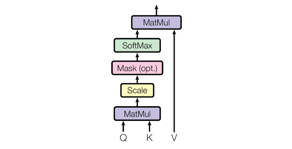
Mathematically, the attention scores are computed as

$$\text{Attention}(\mathbf{Q}, \mathbf{K}, \mathbf{V}) = \text{softmax}\left(\frac{\mathbf{Q}\mathbf{K}^T}{\sqrt{d_k}}\right) \mathbf{V}$$

where

• $\mathbf{Q} \in \mathbb{R}^{n \times d_k}$, $\mathbf{K} \in \mathbb{R}^{m \times d_k}$, $\mathbf{V} \in \mathbb{R}^{m \times d_v}$
• $n$ = number of queries (e.g., sequence length in self-attention)
• $m$ = number of key-value pairs
• $d_k$ = dimension of keys and queries
• $d_v$ = dimension of values
• $\sqrt{d_k}$ is a scaling factor to prevent large dot products from pushing gradients into regions of small magnitude (due to the softmax function).

Multi-Head Attention

While single-head attention is powerful, multi-head attention allows the model to jointly attend to information from different representation subspaces. Instead of computing attention once, the Transformer down-projects the query, key, and value matrices into $h$ smaller matrices (heads), computes attention in parallel, and concatenates the results.

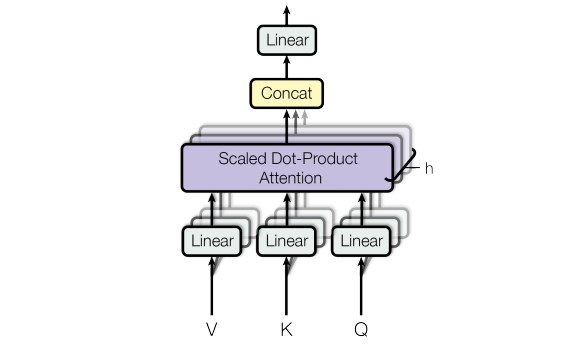
Essentially, this block proceeds as follows:

1. Split into heads

$$\mathbf{Q}_i = \mathbf{Q} \mathbf{W}_i^Q \quad \mathbf{K}_i = \mathbf{K} \mathbf{W}_i^K \quad \mathbf{V}_i = \mathbf{V} \mathbf{W}_i^V \quad \text{for} \quad i = 1, \dots, h$$

where $\mathbf{W}_i^Q, \mathbf{W}_i^K, \mathbf{W}_i^V \in \mathbb{R}^{d_{\text{model}} \times d_k}$ are learned projection matrices, and $d_k = d_{\text{model}} / h$.

2. Compute attention for each head

$$\text{head}_i = \text{Attention}(\mathbf{Q}_i, \mathbf{K}_i, \mathbf{V}_i)$$

3. Concatenate and project

$$\text{MultiHead}(\mathbf{Q}, \mathbf{K}, \mathbf{V}) = \text{Concat}(\text{head}_1, ..., \text{head}_h) \mathbf{W}^O$$

where $\mathbf{W}^O \in \mathbb{R}^{d_{\text{model}} \times d_{\text{model}}}$ is a final projection matrix.

Input Embeddings and Positional Encoding

Before processing, input tokens are converted into dense vector representations via:

1. Token Embeddings: A learned embedding matrix $\mathbf{E} \in \mathbb{R}^{|\mathcal{V}| \times d_{\text{model}}}$, where $|\mathcal{V}|$ is the vocabulary size.
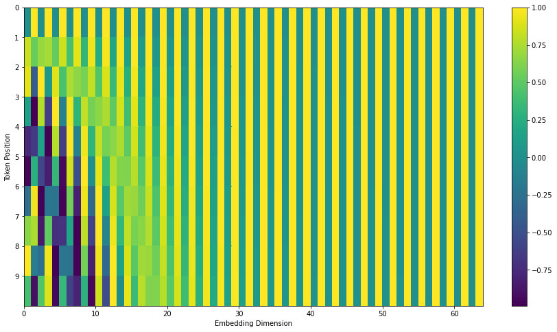
2. Positional Encodings: Since Transformers lack recurrence, they use positional encodings to inject sequence order information. The original paper uses sinusoidal functions:

$$PE_{(pos, 2i)} = \sin\left(\frac{pos}{10000^{2i/d_{\text{model}}}}\right)$$

$$PE_{(pos, 2i+1)} = \cos\left(\frac{pos}{10000^{2i/d_{\text{model}}}}\right)$$

where $pos$ is the position and $i$ is the dimension index.

The final input embedding is then defined as

$$\mathbf{X} = \mathbf{E} + \mathbf{PE}$$

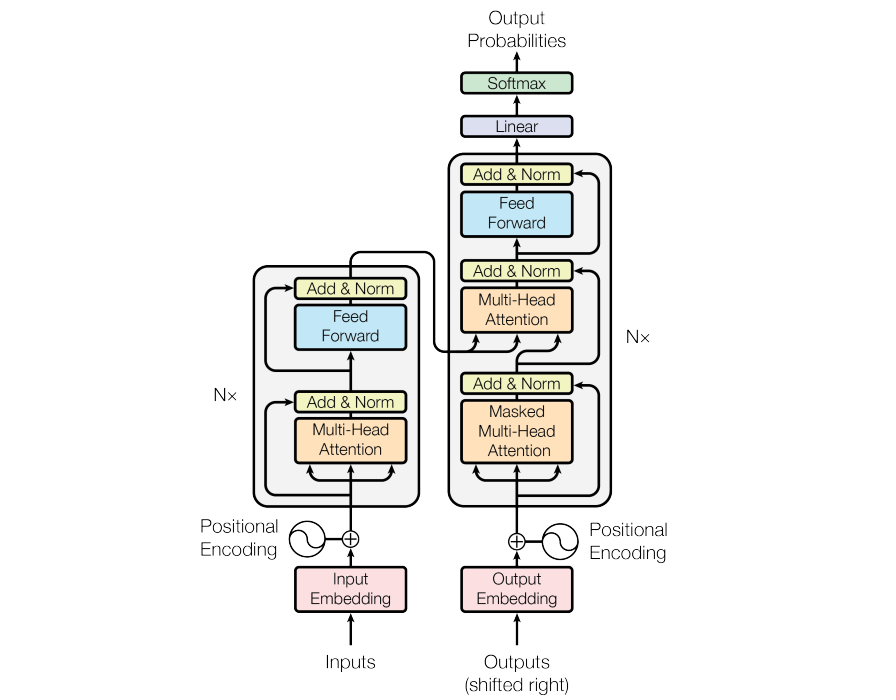
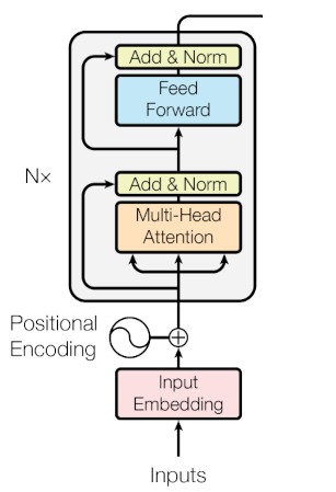
The Encoder Layer

The Transformer encoder consists of a stack of identical layers, each containing two main sub-layers:

1. Multi-Head Scaled Dot-Product Self-Attention
2. Position-Wise Feed-Forward Network (FFN)

Additionally, residual connections and layer normalization are applied around each sub-layer to stabilize training.

Multi-Head Scaled Dot-Product Self-Attention

In the encoder, self-attention means that $\mathbf{Q}, \mathbf{K}, \mathbf{V}$ are all derived from the same input sequence.

For an input matrix $\mathbf{X} \in \mathbb{R}^{n \times d_{\text{model}}}$ (where $n$ is the sequence length):

$$\mathbf{Q} = \mathbf{X} \mathbf{W}^Q, \quad \mathbf{K} = \mathbf{X} \mathbf{W}^K, \quad \mathbf{V} = \mathbf{X} \mathbf{W}^V$$

The multi-head attention output is:

$$\mathbf{Z} = \text{MultiHead}(\mathbf{Q}, \mathbf{K}, \mathbf{V}) + \mathbf{X}$$

(Note the residual connection)

After the attention sub-layer, layer normalization is applied to stabilize training.

$$\text{LayerNorm}(\mathbf{Z}) = \frac{\mathbf{Z} - \mu}{\sigma} \odot \gamma + \beta$$

where

• $\mu, \sigma$ are the mean and standard deviation of $\mathbf{Z}$ (computed per feature across the sequence).
• $\gamma, \beta$ are learned scale and shift parameters.

Position-Wise Feed-Forward Network (FFN)

The Position-Wise Feed-Forward Network applies a two-layer MLP to each position separately and identically, such that

$$\text{FFN}(\mathbf{x}) = \text{ReLU}(\mathbf{x} \mathbf{W}_1 + \mathbf{b}_1) \mathbf{W}_2 + \mathbf{b}_2$$

where

• $\mathbf{W}_1 \in \mathbb{R}^{d_{\text{model}} \times d_{\text{ff}}}$, $\mathbf{W}_2 \in \mathbb{R}^{d_{\text{ff}} \times d_{\text{model}}}$
• $d_{\text{ff}}$ is typically larger than $d_{\text{model}}$

The FFN output is again combined with a residual connection and layer normalization, such that

$$\mathbf{Y} = \text{FFN}(\text{LayerNorm}(\mathbf{Z})) + \text{LayerNorm}(\mathbf{Z})$$

Summary

The full encoder layer can be summarized as:

1. Multi-Head Scaled Dot-Product Self-Attention

$$\mathbf{Z} = \text{MultiHead}(\mathbf{Q}, \mathbf{K}, \mathbf{V}) + \mathbf{X}$$

2. Layer Normalization:

$$\mathbf{Z}_{\text{norm}} = \text{LayerNorm}(\mathbf{Z})$$

3. Position-Wise Feed-Forward Network

$$\mathbf{Y} = \text{FFN}(\mathbf{Z}_{\text{norm}}) + \mathbf{Z}_{\text{norm}}$$

4. Final Layer Normalization (optional in some variants).

The output $\mathbf{Y}$ is then passed to the next encoder layer or, in an encoder-decoder model, to the decoder via cross-attention.

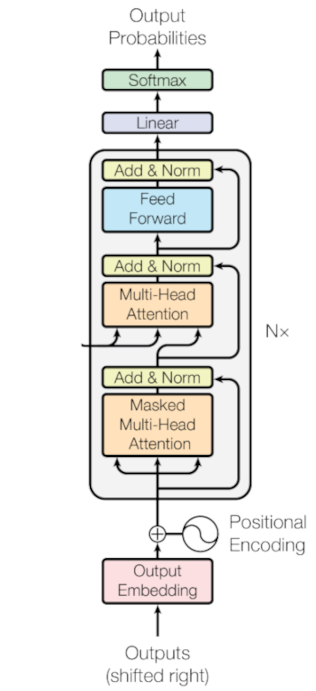
The Decoder Layer

The decoder shares many components with the encoder but introduces two key modifications:

1. Masked Multi-Head Scaled Dot-Product Self-Attention to prevent looking ahead in autoregressive tasks.
2. Multi-Head Scaled Dot-Product Cross-Attention to attend to encoder outputs.

Masked Multi-Head Scaled Dot-Product Self-Attention

In autoregressive tasks (e.g., language generation), the decoder must not attend to future tokens. This is enforced via a look-ahead mask applied to the attention scores before softmax.

The mask matrix $\mathbf{M} \in \mathbb{R}^{n \times n}$ is defined as

$$\mathbf{M}_{ij} = \begin{cases} 0 & \text{if } i \leq j \\ -\infty & \text{if } i > j \end{cases}$$

Given the attention scores $\mathbf{A}$ calculated as

$$\mathbf{A} = \frac{\mathbf{Q} \mathbf{K}^T}{\sqrt{d_k}}$$

The masked attention scores are derived as

$$\mathbf{A}_{\text{masked}} = \mathbf{A} + \mathbf{M}$$

After applying softmax, future positions have zero attention weight.

Multi-Head Scaled Dot-Product Cross-Attention

After masked self-attention, the decoder performs cross-attention, where

• Queries ($\mathbf{Q}$) come from the decoder’s previous layer output
• Keys ($\mathbf{K}$) and Values ($\mathbf{V}$) come from the encoder’s final output

$$\mathbf{Z}_{\text{cross}} = \text{MultiHead}(\mathbf{Q}_{\text{dec}}, \mathbf{K}_{\text{enc}}, \mathbf{V}_{\text{enc}})$$

where:

• $\mathbf{Q}_{\text{dec}} = \mathbf{Y}_{\text{prev}} \mathbf{W}^Q$ (from decoder)
• $\mathbf{K}_{\text{enc}} = \mathbf{Y}_{\text{enc}} \mathbf{W}^K$ (from encoder)
• $\mathbf{V}_{\text{enc}} = \mathbf{Y}_{\text{enc}} \mathbf{W}^V$ (from encoder)

Summary

The full decoder layer consists of:

1. Masked Multi-Head Scaled Dot-Product Self-Attention

$$\mathbf{Z}_1 = \text{MultiHead}_{\text{masked}}(\mathbf{Q}, \mathbf{K}, \mathbf{V}) + \mathbf{X}$$

2. Layer Normalization

$$\mathbf{Z}_{1,\text{norm}} = \text{LayerNorm}(\mathbf{Z}_1)$$

3. Multi-Head Scaled Dot-Product Cross-Attention

$$\mathbf{Z}_2 = \text{MultiHead}(\mathbf{Z}_{1,\text{norm}} \mathbf{W}^Q, \mathbf{Y}_{\text{enc}} \mathbf{W}^K, \mathbf{Y}_{\text{enc}} \mathbf{W}^V) + \mathbf{Z}_{1,\text{norm}}$$

4. Layer Normalization

$$\mathbf{Z}_{2,\text{norm}} = \text{LayerNorm}(\mathbf{Z}_2)$$

5. Position-Wise Feed-Forward Network

$$\mathbf{Y} = \text{FFN}(\mathbf{Z}_{2,\text{norm}}) + \mathbf{Z}_{2,\text{norm}}$$

Encoder, Decoder, Encoder-Decoder

The Transformer architecture is highly modular, allowing for three main variants:

• Encoder-Only Models (e.g., BERT)
• Decoder-Only Models (e.g., GPT)
• Encoder-Decoder Models (e.g., original Transformer, T5)

Encoder-Only Models

Encoder-Only Models such as BERT are built of a stack of transformer encoder layers, utilizing the bidirectional self-attention, allowing them to process input sequence in full context.

Training happens in 2 phases:

• Pre-Training: The model learns language patterns via 2 objectives
  • Masked Language Modelling (MLM): Randomly mask 15% of input tokens and predict them.
  • Next Sentence Prediction (NSP): Predict whether two sentences are consecutive.
• Fine-Tuning: The pre-trained model is adapted for downstream tasks (e.g. classifcation, NER) by adding an additional task-specific layer suited for the downstream task.

These models excel at understanding context and are widely used for tasks requiring deep semantic analysis.

Decoder-Only Models

Decoder-Only Models such as GPT rely on a stack of transformer decoder layers, operating without an encoder. Their key feature is masked (autoregressive) self-attention, which restricts attention to previous tokens only, ensuring predictions are made strictly left-to-right. Since there’s no encoder, they lack cross-attention but excel at generative tasks by modeling sequential dependencies.

Training follows a two-step process:

• Pre-Training
  • Objective: Causal Language Modeling (CLM) - predict next token given previous tokens.
  • Data: Large-scale unlabelled text (e.g., web, books).
• Fine-Tuning
  • Supervised: Adapt to tasks (e.g., summarization) via labeled (prompt, response) pairs.
  • Instruction-Tuning: Train on diverse (instruction, output) data for zero-shot generalization.
  • RLHF (Optional): Align with human preferences via reinforcement learning.

These models thrive in generative applications, including:

• Text generation (stories, code, poetry)
• Chatbots and dialogue systems
• Autocomplete and suggestion tools
• Few-shot learning (adapting to new tasks via prompt engineering)

Their strength lies in coherent, context-aware generation, making them ideal for open-ended tasks where creativity or fluid responses are needed.

Encoder-Decoder Models

Encoder-Decoder Models such as the original Transformer implementation, or T5 combine two transformer stacks: an encoder that processes input sequences and a decoder that generates output sequences while attending to the encoder’s representations via cross-attention.

This architecture is designed for sequence-to-sequence (seq2seq) tasks, where the goal is to transform one sequence into another, such as translating languages or summarizing text.

During training, the model learns in a supervised manner, typically using teacher forcing, which means that the decoder receives the ground-truth previous token (not its own prediction) to ensure stable learning.

At inference time, however, the decoder generates tokens autoregressively, feeding its own predictions back as input for the next step.

These models excel in tasks requiring transformation or generation from structured input.

• Machine translation (e.g., English to German)
• Text summarization (condensing long documents)
• Context-aware question answering (extracting answers from a given passage)
• Data-to-text generation (converting tables or structured data into natural language)

Their ability to map complex inputs to structured outputs makes them versatile for applications where both understanding and generation are critical.

Conclusion

The Transformer architecture revolutionized AI by replacing recurrence with self-attention, enabling parallel processing and superior performance in NLP.

Its Query-Key-Value mechanism dynamically weighs input relevance, while multi-head attention captures diverse relationships.

With encoder-only (BERT), decoder-only (GPT), and encoder-decoder (T5) variants, Transformers power everything from translation to generation.