Artificial Neural Network Backpropagation

Artificial Neural Networks are the backbone of modern machine learning, enabling breakthroughs in computer vision, natural language processing and reinforcement learning. At the core of their training lies backpropagation, an algorithm that efficiently computes gradients of the loss function with respect to the network's parameters.

To truly understand backpropagation, we must first establish a strong foundation in derivatives, the chain rule, loss functions and gradient descent.

In this blog post, we explore these concepts, culminating in a detailed explanation of how backpropagation works, including the delta backpropgation update rule and its mathematical formulation.

Derivatives — The Foundation

A derivative is a function $f(x)$ with respect to $x$, denoted $\frac{df}{dx}$ or $f'(x)$, measures the rate at which the function's output changes as its input changes.

$$\frac{df}{dx} = f'(x) = \lim_{h \rightarrow 0} \frac{f(x+h) - f(x)}{h}$$

In artificial neural networks, we deal with multivariate functions, in which the output depends on multiple inputs (parameters). There, we use partial derivatives to measure how the output changes with respect to each individual parameter while keeping others constant.

For a function $f(\mathbf{x})$ where $\mathbf{x} = [x_1, x_2, \dots, x_n]^T$, the partial derivative with respect to $x_i$ is:

$$\frac{\partial f}{\partial x_i} = \lim_{h \to 0} \frac{f(x_1, \dots, x_i + h, \dots, x_n) - f(x_1, \dots, x_n)}{h}$$

The gradient of $f$ is the vector of all partial derivatives:

$$\nabla f = \left[ \frac{\partial f}{\partial x_1}, \frac{\partial f}{\partial x_2}, \dots, \frac{\partial f}{\partial x_n} \right]^T$$

Artificial Neural Networks learn by adjusting their parameters (weights $\mathbf{W}$ and biases $\mathbf{b}$) to minimize a loss function $L$. To do this, we need to know how much each parameter contributes to the loss. The gradient $\nabla L$ tells us the direction and magnitude of adjustment needed for each parameter.

Chain Rule — The Backbone of Backpropagation

The chain rule is a fundamental concept in calculus which allows to compute derivatives of composite functions. If a function $y$ depends on a function $u$, which in turn depends on some input $x$, then

$$\frac{dy}{dx} = \frac{dy}{du} \cdot \frac{du}{dx}$$

In artificial neural networks, computations are layered, meaning the output of one layer is the input to the next. The chain rule allows us to propagate gradients backward through these layers efficiently.

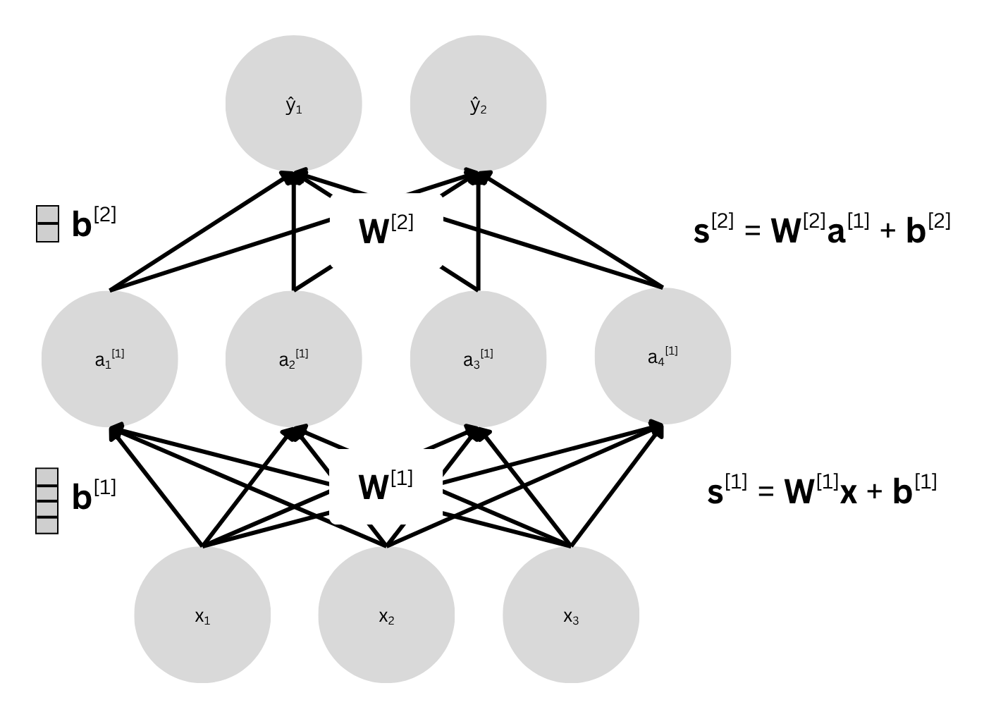
Consider a two-layer artificial neural network with

• Input vector $\mathbf{x} \in \mathbb{R}^3$
• Weight matrices $\mathbf{W}^{[1]} \in \mathbb{R}^{4 \times 3}, \mathbf{W}^{[2]} \in \mathbb{R}^{2 \times 4}$
• Bias vectors $\mathbf{b}^{[1]} \in \mathbb{R}^{4}, \mathbf{b}^{[2]} \in \mathbb{R}^{2}$
• Pre-activations $\mathbf{s}^{[1]} = \mathbf{W}^{[1]} \mathbf{x} + \mathbf{b}^{[1]}$
• Activations $\mathbf{a}^{[1]} = \sigma(\mathbf{s}^{[1]})$ (where $\sigma$ is an activation function, e.g., ReLU or sigmoid)
• Pre-activations $\mathbf{s}^{[2]} = \mathbf{W}^{[2]} \mathbf{a}^{[1]} + \mathbf{b}^{[2]}$
• Final output $\hat{\mathbf{y}} = \sigma(\mathbf{s}^{[2]})$

The prediction $\hat{\mathbf{y}}$ depends on $\mathbf{s}^{[2]}$ which depends on $\mathbf{a}^{[1]}$, which depends on $\mathbf{s}^{[1]}$ and so on.

Loss Functions — Quantifying Prediction Error

A loss function (or cost function) measures the discrepancy between the predicted outputs $\hat{\mathbf{y}}$ of a neural network and the true target values $\mathbf{y}$. The primary objective during training is to minimize this loss by adjusting the model's parameters using gradient-based optimization techniques.

Regression: Mean Squared Error (MSE)

For regression problems, where the goal is to predict continuous numerical values, the Mean Squared Error (MSE) is a commonly used loss function.

The MSE loss is defined as:

$$L = \frac{1}{2} \sum_{i=1}^n (\hat{y}_i - y_i)^2$$

where $\hat{y}_i$ denotes the predicted value for the $i$-th sample, $y_i$ represents the true target value for the $i$-th sample, and $n$ defines the number of samples.

The squared term of MSE penalizes larger errors more severely, making the model sensitive to outliers.

Mean Squared Error – Derivation

We assume the target $y$ is a continuous variable corrupted by Gaussian noise, hence the model would be given as $y = f(x) + \epsilon$, where $\epsilon \sim \mathcal{N}(0, \sigma^2)$.

1. Likelihood: The probability of observing $y_i$ given $\hat{y}_i$ (the prediction) is

$$p(y_i | \hat{y}_i) = \frac{1}{\sqrt{2\pi\sigma^2}} \exp\left(-\frac{(y_i - \hat{y}_i)^2}{2\sigma^2}\right)$$

2. Negative Log-Likelihood (NLL): To maximize likelihood, we minimize Negative Log-Likelihood

$$-\log p(y_i | \hat{y}_i) = \frac{(y_i - \hat{y}_i)^2}{2\sigma^2} + \text{const.}$$

3. Sum over all samples: The total loss is

$$L = \sum_{i=1}^n \frac{(y_i - \hat{y}_i)^2}{2\sigma^2}$$

4. Simplification: If we assume $\sigma = 1$ (or absorb it into a constant), we get:

$$L = \frac{1}{2} \sum_{i=1}^n (y_i - \hat{y}_i)^2$$

Hence, MSE arises from maximizing the likelihood under Gaussian noise.

The squared term penalizes large errors more heavily, which is desirable when outliers are rare (Gaussian assumption).

Binary Classification: Binary Cross-Entropy

For binary classification, where the output is a probability between 0 and 1, the Binary Cross-Entropy (BCE) loss is used.

The BCE loss is defined as:

$$L = - \frac{1}{n} \sum_{i=1}^n \left[ y_i \log(\hat{y}_i) + (1 - y_i) \log(1 - \hat{y}_i) \right]$$

where $\hat{y}_i$ is the predicted probability of class 1 (output of a sigmoid function), and $y_i \in \{0, 1\}$ represents the true binary label.

The logarithmic penalty means incorrect predictions with high confidence (e.g., $\hat{y}_i \approx 1$ when $y_i = 0$) are penalized heavily.

Binary Cross-Entropy – Derivation

We assume the target $y \in \{0, 1\}$ is a Bernoulli random variable, hence the model would be defined as $p(y_i = 1 | x_i) = \hat{y}_i$, where $\hat{y}_i \in (0, 1)$ (output of a sigmoid).

1. Likelihood: The probability of observing $y_i$ is

$$p(y_i | \hat{y}_i) = \hat{y}_i^{y_i} (1 - \hat{y}_i)^{1 - y_i}$$

2. Negative Log-Likelihood (NLL): To maximize likelihood, we minimize Negative Log-Likelihood

$$-\log p(y_i | \hat{y}_i) = -y_i \log \hat{y}_i - (1 - y_i) \log (1 - \hat{y}_i)$$

3. Sum over all samples: The total loss is

$$L = -\sum_{i=1}^n \left[ y_i \log \hat{y}_i + (1 - y_i) \log (1 - \hat{y}_i) \right]$$

4. Normalization: Divide by $n$ to average over samples:

$$L = -\frac{1}{n} \sum_{i=1}^n \left[ y_i \log \hat{y}_i + (1 - y_i) \log (1 - \hat{y}_i) \right].$$

Hence, BCE arises from maximizing the likelihood under a Bernoulli assumption.

The log terms heavily penalize confident wrong predictions (e.g., $\hat{y}_i \approx 1$ when $y_i = 0$).

Multi-Class Classification: Categorical Cross-Entropy

For multi-class classification, where each sample belongs to one of $C$ classes, the Categorical Cross-Entropy (CCE) loss is used.

The CCE loss is defined as:

$$L = - \frac{1}{n} \sum_{i=1}^n \sum_{j=1}^C y_{i,j} \log(\hat{y}_{i,j})$$

where $\hat{y}_{i,j}$ is the predicted probability for class $j$ (output of a softmax function), and $y_{i,j}$ is the true one-hot encoded label (1 if sample $i$ belongs to class $j$, else 0).

The softmax normalization ensures predicted probabilities sum to 1.

It's important to note that only the true class contributes to the loss (other terms vanish due to $y_{i,j} = 0$).

Categorical Cross-Entropy – Derivation

We assume the target $y$ is a one-hot encoded vector for $C$ classes, drawn from a categorical distribution, hence the model would be given as $p(y_i = j | x_i) = \hat{y}_{i,j}$, where $\sum_{j=1}^C \hat{y}_{i,j} = 1$ (output of a softmax).

1. Likelihood: The probability of observing $y_i$ (one-hot) is

$$p(y_i | \hat{y}_i) = \prod_{j=1}^C \hat{y}_{i,j}^{y_{i,j}}$$

2. Negative Log-Likelihood (NLL): To maximize likelihood, we minimize Negative Log-Likelihood

$$-\log p(y_i | \hat{y}_i) = -\sum_{j=1}^C y_{i,j} \log \hat{y}_{i,j}$$

3. Sum over all samples: The total loss is

$$L = -\sum_{i=1}^n \sum_{j=1}^C y_{i,j} \log \hat{y}_{i,j}$$

4. Normalization: Divide by $n$ to average over samples

$$L = -\frac{1}{n} \sum_{i=1}^n \sum_{j=1}^C y_{i,j} \log \hat{y}_{i,j}$$

Hence, CCE arises from maximizing the likelihood under a categorical distribution.

Only the true class $j$ (where $y_{i,j} = 1$) contributes to the loss.

The softmax ensures valid probabilities, and the log penalizes incorrect confident predictions.

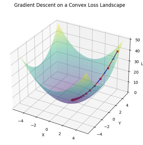
Gradient Descent — Optimizing the Loss Function

Gradient Descent is an iterative optimization algorithm used to minimize a loss function $L(\theta)$ by adjusting the parameters $\theta$ in the direction that reduces the loss the most.

The parameter $\theta$ is updated as follows

$$\theta \leftarrow \theta - \eta \frac{\partial L}{\partial \theta}$$

where $\eta$ (learning rate) is a small positive scalar (e.g., $0.01, 0.001$) that controls the step size, and $\frac{\partial L}{\partial \theta}$ is the gradient of the loss function with respect to $\theta$.

• Gradient Direction: The gradient $\frac{\partial L}{\partial \theta}$ points in the direction of the steepest increase of $L$, so we move in the opposite direction to minimize the loss.
• Learning Rate ($\eta$): If $\eta$ is too large, the algorithm may overshoot the minimum; if too small, convergence will be slow.
• Iterative Process: The update is repeated until the loss stabilizes or the gradient becomes very small.

Backpropagation — Efficient Gradient Computation

Backpropagation is an algorithm that computes the gradient of the loss function with respect to the weights and biases of the neural network. It does this by applying the chain rule to propagate gradients through the network.

The Forward Pass

Before we are able to calculate gradients of the Loss function wrt to the parameters, we must first pass the data $x$ through the network to get the current prediction, from which we can then work backwards.

Hence, given $\mathbf{x}$, we compute

1. $\mathbf{s}^{[1]} = \mathbf{W}^{[1]} \mathbf{x} + \mathbf{b}^{[1]}$
2. $\mathbf{a}^{[1]} = \sigma(\mathbf{s}^{[1]})$
3. $\mathbf{s}^{[2]} = \mathbf{W}^{[2]} \mathbf{a}^{[1]} + \mathbf{b}^{[2]}$
4. $\hat {\mathbf{y}} = \sigma(\mathbf{s}^{[2]})$
5. Compute loss $L(\hat{\mathbf{y}}, \mathbf{y})$, assume regression task with MSE loss $L = \frac{1}{2} \sum_{i=1}^n (\hat{y}_i - y_i)^2$

This will yield the loss (prediction error) of the model given its current parameter setup. From this we can perform the backward pass, calculating the gradients of the loss with respect to the parameter weight matrices $\mathbf{W}$ and bias vectors $\mathbf{b}$.

The Backward Pass

In order to update our parameters, we have to find $\frac{\partial L}{\partial \mathbf{W}^{[1]}}, \frac{\partial L}{\partial \mathbf{b}^{[1]}}, \frac{\partial L}{\partial \mathbf{W}^{[2]}}, \frac{\partial L}{\partial \mathbf{b}^{[2]}}$

Step 1: Gradient of the Loss wrt. Output $\hat{\mathbf{y}}$

$$\frac{\partial L}{\partial \hat{\mathbf{y}}} = \hat{\mathbf{y}} - \mathbf{y}$$

Step 2: Gradient of the Loss wrt. Pre-Activation $\mathbf{s}^{[2]}$

Using the chain rule:

$$\frac{\partial L}{\partial \mathbf{s}^{[2]}} = \frac{\partial L}{\partial \hat{\mathbf{y}}} \odot \sigma'(\mathbf{s}^{[2]})$$

where $\odot$ is element-wise multiplication and $\sigma'$ is the derivative of the activation function.

Step 3: Gradient of the Loss wrt. Weights $\mathbf{W}^{[2]}$

$$\frac{\partial L}{\partial \mathbf{W}^{[2]}} = \frac{\partial L}{\partial \mathbf{s}^{[2]}} \mathbf{a}^{[1]^T}$$

Step 4: Gradient of the Loss wrt. Bias $\mathbf{b}^{[2]}$

$$\frac{\partial L}{\partial \mathbf{b}^{[2]}} = \frac{\partial L}{\partial \mathbf{s}^{[2]}}$$

Step 5: Gradient of the Loss wrt. Activation $\mathbf{a}^{[1]}$

$$\frac{\partial L}{\partial \mathbf{a}^{[1]}} = \mathbf{W}^{[2]^T} \frac{\partial L}{\partial \mathbf{s}^{[2]}}$$

Step 6: Gradient of the Loss wrt. Pre-Activation $\mathbf{s}^{[1]}$

$$\frac{\partial L}{\partial \mathbf{s}^{[1]}} = \frac{\partial L}{\partial \mathbf{a}^{[1]}} \odot \sigma'(\mathbf{s}^{[1]})$$

Step 7: Gradient of the Loss wrt. Weights $\mathbf{W}^{[1]}$

$$\frac{\partial L}{\partial \mathbf{W}^{[1]}} = \frac{\partial L}{\partial \mathbf{s}^{[1]}} \mathbf{x}^T$$

Step 8: Gradient of the Loss wrt. Bias $\mathbf{b}^{[1]}$

$$\frac{\partial L}{\partial \mathbf{b}^{[1]}} = \frac{\partial L}{\partial \mathbf{s}^{[1]}}$$

The Parameter Updates

Once all gradients are computed, we update the parameters using gradient descent:

$$\mathbf{W}^{[1]} \leftarrow \mathbf{W}^{[1]} - \eta \frac{\partial L}{\partial \mathbf{W}^{[1]}}$$

$$\mathbf{b}^{[1]} \leftarrow \mathbf{b}^{[1]} - \eta \frac{\partial L}{\partial \mathbf{b}^{[1]}}$$

$$\mathbf{W}^{[2]} \leftarrow \mathbf{W}^{[2]} - \eta \frac{\partial L}{\partial \mathbf{W}^{[2]}}$$

$$\mathbf{b}^{[2]} \leftarrow \mathbf{b}^{[2]} - \eta \frac{\partial L}{\partial \mathbf{b}^{[2]}}$$

$\delta$ Delta Backpropagation — Recursive $\delta$ Errors

The delta backpropagation algorithm is essentially the same as the standard backpropagation algorithm but is often framed in terms of "deltas" (errors) propagated backward through the network.

Deriving the Delta Backpropagation Formulation

The derivations of the previous section already compute gradients efficiently by applying the chain rule in a structured way. A notable observation however is that the gradients for the weights and biases at each layer depend on two key terms:

1. The derivative of the loss with respect to the pre-activation ($\frac{\partial L}{\partial \mathbf{s}^{[l]}}$), which incorporates the error signal.
2. The derivative of the activation function ($\sigma'(\mathbf{s}^{[l]})$), which modulates how the error propagates backward.

The delta formulation of backpropagation reframes these computations in terms of error signals ($\delta^{[l]}$) to emphasize the recursive nature of gradient propagation. Instead of treating $\frac{\partial L}{\partial \mathbf{s}^{[l]}}$ as an intermediate quantity, we define it explicitly as $\delta^{[l]}$, making the backward pass more intuitive.

Output Layer Delta Error $\delta$

Based on the original derivation, we have

$$\frac{\partial L}{\partial \mathbf{s}^{[2]}} = \frac{\partial L}{\partial \hat{\mathbf{y}}} \odot \sigma'(\mathbf{s}^{[2]})$$

Since $\frac{\partial L}{\partial \hat{\mathbf{y}}} = \hat{\mathbf{y}} - \mathbf{y}$ (from MSE loss), we can write:

$$\delta^{[2]} = (\hat{\mathbf{y}} - \mathbf{y}) \odot \sigma'(\mathbf{s}^{[2]})$$

This is the output layer delta, representing how much the final layer's pre-activation contributed to the loss.

Hidden Layer Delta Error $\delta$

The gradient of the loss with respect to the hidden layer's pre-activation is:

$$\frac{\partial L}{\partial \mathbf{s}^{[1]}} = \frac{\partial L}{\partial \mathbf{a}^{[1]}} \odot \sigma'(\mathbf{s}^{[1]})$$

But $\frac{\partial L}{\partial \mathbf{a}^{[1]}}$ is computed as:

$$\frac{\partial L}{\partial \mathbf{a}^{[1]}} = \mathbf{W}^{[2]^T} \frac{\partial L}{\partial \mathbf{s}^{[2]}} = \mathbf{W}^{[2]^T} \delta^{[2]}$$

Thus, the hidden layer delta is:

$$\delta^{[1]} = \left( \mathbf{W}^{[2]^T} \delta^{[2]} \right) \odot \sigma'(\mathbf{s}^{[1]})$$

This shows how the error from the output layer is propagated backward to the hidden layer, weighted by $\mathbf{W}^{[2]^T}$ and modulated by the activation derivative.

Gradient Computation Using Deltas

Now, the gradients for the weights and biases can be expressed directly in terms of the deltas:

• $\mathbf{W}^{[2]}$ and $\mathbf{b}^{[2]}$

$$\frac{\partial L}{\partial \mathbf{W}^{[2]}} = \delta^{[2]} \mathbf{a}^{[1]^T} \quad \frac{\partial L}{\partial \mathbf{b}^{[2]}} = \delta^{[2]}$$

• For $\mathbf{W}^{[1]}$ and $\mathbf{b}^{[1]}$:

$$\frac{\partial L}{\partial \mathbf{W}^{[1]}} = \delta^{[1]} \mathbf{x}^T \quad \frac{\partial L}{\partial \mathbf{b}^{[1]}} = \delta^{[1]}$$

Why the Delta Formulation?

The delta formulation is not just a notational change—it highlights the recursive structure of backpropagation:

• Error Propagation: The delta at layer $l$ ($\delta^{[l]}$) depends on the delta from layer $l+1$ ($\delta^{[l+1]}$), weighted by the transpose of the connecting weights ($\mathbf{W}^{[l+1]^T}$).
• Modulation by Activation Derivative: The derivative of the activation function ($\sigma'(\mathbf{s}^{[l]})$) scales the propagated error, ensuring that the gradient respects the nonlinearity of the network.
• Efficiency: By defining $\delta^{[l]}$ explicitly, we avoid recomputing intermediate terms, making the backward pass more computationally efficient.

The delta terms encapsulate the local gradient information at each layer, making the algorithm both intuitive and scalable.

Conclusion

Backpropagation is the cornerstone of training artificial neural networks, enabling them to learn from data by efficiently computing gradients and updating parameters.

By leveraging the chain rule, backpropagation propagates errors backward through the network, allowing us to adjust weights and biases in a way that minimizes prediction errors.